Tutorial

This is an overview of the iode library. It is not intended to be a fully comprehensive manual. It is mainly dedicated to help new users to familiarize with it and others to remind essentials.

LEC language

This tutorial is a practical introduction to the LEC language (Langage Econometrique Condense), the formula language used in IODE.

You will learn how to:

write valid LEC expressions
use variables, scalars, and constants
work with lags, leads, and fixed periods
use mathematical and time functions
write equations with :=

For a full explanation of the syntax and features, see the The LEC Language section.

What Is LEC?

LEC is designed for formulas involving time series. It is used in equations, identities, and table formulas.

Example 1:

\[C_t = a + b \frac{Y_t}{P_t} + c C_{t-1}\]

LEC form:

C := a + b * Y / P + c * C[-1]

Example 2:

\[\ln(Q_t) = a\ln(K_t) + (1-a)\ln(L_t) + c t + b\]

LEC form:

ln Q := a * ln K + (1 - a) * ln L + c * t + b

Basic Building Blocks

Numeric constants

You can use integers, floating-point numbers, and scientific notation:

2
0.125
1.2E-03

Language constants

LEC provides three predefined constants:

pi
e
euro

Temporal constants and t

Temporal constants represent periods:

1990Y1
1970Q4
2010M11

The symbol t is the index of the current execution period.

Example:

X * (t < 1990Y1) + Y * (t >= 1990Y1)

This formula returns X before 1990Y1 and Y from 1990Y1 onward.

Variables and Scalars

Variables

Variables are time series and must start with an uppercase letter.

Valid examples:

A
B_PNB
A123456789

Invalid examples:

_A1
1A34
z_AV
A-2

Scalars

Scalars are single values and must start with a lowercase letter.

Valid examples:

a
c1
a_123456789

Invalid examples:

_a1
1A34
Z_av

Time Indexing (Lag, Lead, Fixed Period)

You can shift any expression in time:

lag: expr[-n]
lead: expr[+n]
fixed period: expr[1990Y1]

Examples:

PNB[-1]
PNB[+1]
PNB[1990Y1]

Important rule:

once a fixed period is applied, additional lags/leads no longer change that part

Examples:

(A + B[+1])[-2]          => A[-2] + B[-1]
(A[70Y1] + B)[-1][-2]    => A[70Y1] + B[-3]

Algebraic and Logical Operators

Algebraic operators:

+, -, *, /, **

Logical operators:

not or !
or
and
<, <=, =, != (or <>), >=, >

Logical expressions evaluate to 1 (true) or 0 (false).

Examples:

X and !Y
Z < 1 * 3
X = 0 and Y = 0 or Z = 2

Mathematical Functions

Common functions:

ln(expr), log([base], expr), exp([base,] expr)
max(...), min(...), lsum(...)
abs(expr), sqrt(expr), round(expr [, n])
if(cond, value_if_true, value_if_false)

Single-argument functions can be written without parentheses:

ln X + 2
d X

is equivalent to:

ln(X) + 2
d(X)

Conditional example:

if(t < 1992Y1, 2, X)

Time Functions

LEC includes many time-series operators.

Most used ones (by default k = 1):

l([k,] expr): lag expression
d([k,] expr): period difference
r([k,] expr): period ratio
dln([k,] expr): difference of logs
grt([k,] expr): growth rate in %
ma([k,] expr) / mavg([k,] expr): moving average

Examples:

d(PNB)
dln(X)
grt(4, X)
ma(3, X)

Range functions:

sum([from,[to,]] expr)
prod([from,[to,]] expr)
mean([from,[to,]] expr)
vmax([from,[to,]] expr)
vmin([from,[to,]] expr)

Examples:

sum(0, t, X)
mean(t - 3, t, X)
vmax(1970Y1, 1990Y1, X + Y)

Statistics functions include var, covar, corr, stderr, and stddev.

Special Variable `i` in Sub-Expressions

Inside some time functions (such as sum), the special variable i is the offset between the current formula period and the sub-expression period.

Example:

sum(t-2, t-4, A / (1 - i)**2)

This lets you write dynamic expressions that depend on the internal iteration period.

Lists and Macros

Named lists

Use $LISTNAME to insert a list expression:

A + B + $A + 2

If list A is PNB * c1 + c2, this becomes:

A + B + PNB * c1 + c2 + 2

Computed lists with wildcards

Use single quotes around wildcard patterns:

lsum('A*')
max('*G;*F')

Note: wildcard expansion is resolved at compile time against the current variables workspace.

Comments

Two comment styles are available.

Inline block comments:

A + B + /* first part */ C + D

Trailing comments with ;:

ln Y := c1 + c2 * ln Y[-1] ; free comment

Warning: ; ends the equation. Everything after it is ignored.

Operator Precedence

From lowest to highest priority:

or
and
comparisons (<, <=, =, …)
+ and -
* and /
**
mathematical and time functions

Use parentheses to force evaluation order.

Writing Equations

An equation has the form:

expr1 := expr2

Example:

ln Y := c1 + c2 * ln Z + c3 * ln Y[-1]

The endogenous variable should appear in the equation.

Quick Syntax Reminder

numeric constants      : 2, 2.0, 2.12E2 0.001e-03
temporal constants     : 1990Y1, 80S2, 78Q4, 2003M12
language constants     : pi, e, t
variables              : A, A_1, A123456789
scalars                : a, a_1, x123456789
logical operators      : not expr
                         expr or expr
                         expr and expr
                         expr < expr
                         expr <= expr
                         expr = expr
                         expr != expr
                         expr >= expr
                         expr > expr
algebraic operators    : expr + expr
                         expr - expr
                         expr / expr
                         expr * expr
                         expr ** expr
mathematical functions : -expr
                         +expr
                         log([expr], expr)
                         ln(expr)
                         exp([expr,] expr)
                         max(expr, ...)
                         min(expr, ...)
                         lsum(expr, expr, ...)
                         sin(expr)
                         cos(expr)
                         acos(expr)
                         asin(expr)
                         tan(expr)
                         atan(expr)
                         tanh(expr)
                         sinh(expr)
                         cosh(expr)
                         abs(expr)
                         sqrt(expr)
                         int(expr)
                         rad(expr)
                         if(expr, expr, expr)
                         sign(expr)
                         isan(expr)
                         lmean(expr, ...)
                         lprod(expr, ...)
                         lcount(expr, ...)
                         floor(expr)
                         ceil(expr)
                         round(expr [, n])
                         random(expr)
time functions         : l([expr,] expr)
                         d([expr,] expr)
                         r([expr,] expr)
                         dln([expr,] expr)
                         grt([expr,] expr)
                         ma([expr,] expr)
                         mavg([expr,] expr)
                         vmax([expr,[expr,]] expr)
                         vmin([expr,[expr,]] expr)
                         sum([expr,[expr,]] expr)
                         prod([expr,[expr,]] expr)
                         mean([expr,[expr,]] expr)
                         index([expr,[expr,]] expr1, expr2)
                         acf([expr,[expr,]] expr, expr)
                         var([from [,to],] expr)
                         covar([from [,to],] expr1, expr2)
                         covar0([from [,to],] expr1, expr2)
                         corr([from [,to],] x, y)
                         stderr([expr,[expr,]] expr)
                         stddev([from [,to],] expr)
                         lastobs([from [,to],] expr)
                         interpol(expr)
                         app(expr1, expr2)
                         dapp(expr1, expr2)
lists or macros        : $LISTNAME
lags, leads, periods   : [+n] [-n] [1990Y1]
comments               : /* Comment */
equations              : expr := expr

IODE reports

Purpose And Context

Automation and Scripting: IODE reports use scripting to chain commands and automate tasks, enabling repeatable logic and outputs.
Report File Extension: IODE report files have the extension .rep and are simple text files.
Report File Structure: Report files contain commands (and comments) edited with the graphical user interface (GUI) or any simple text editor.
Modularity: A report can be split into sub-reports. Procedures are user defined functions that can be reused to avoid code duplication and then improve the maintenance.
Content: IODE reports contain commands, functions, macros, LEC expressions and comments.

Running Reports

Reports can be run from the graphical user interface (GUI), the command line (Windows terminal), or programmatically from Python.
Arguments can be passed to the executed report.

Graphical User Interface (GUI)

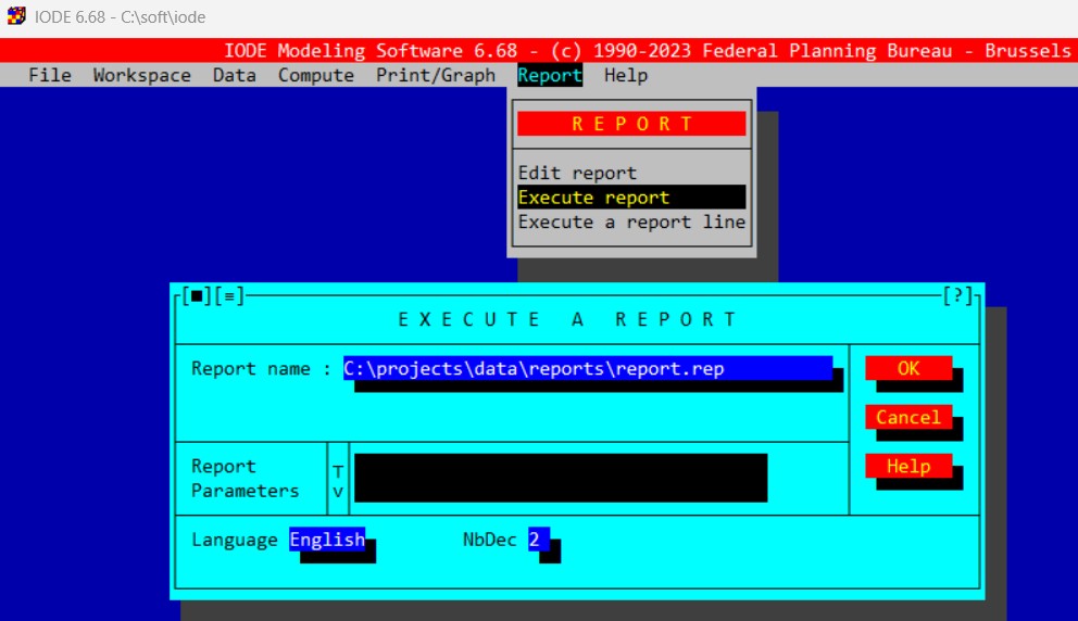
Old Interface: to execute a report, you need to go to the menu Report and click on Execute report.

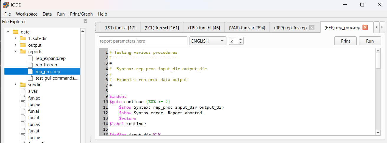
New Interface: to execute a report, you need to double click on the report file in the file explorer (left panel) and then click on the Run button.

Command Line (Windows Terminal)

Open a Windows terminal and run the command:

iodecmd [-nbrun n] [-v] [-y] [-h] reportfile.rep [arg1] ... [argn]

where:

nbrun n: n = number of repetitions of the report execution (default 1)
v: verbose mode (all messages displayed)
y: answer yes to all questions asked during the report execution
h: display the iodecmd options
reportfile.rep arg1 …: IODE report to be executed including its optional arguments

See the section Command Line Interface (iodecmd) for more details.

Python

In Python script, IODE reports are called using the execute_report() function. For example:

import iode as io
first_year = "2010Y1"
last_year = "2070Y1"
convergence = "0.01"
relax = "1.0"
io.execute_report("simulation.rep", [first_year, last_year, convergence, relax])

Modular Report Invocation

Reports can invoke other reports using the $ReportExec reportfile.rep [arg1] … [argn] command for modular and reusable pipelines (see $reportexec for more details).

Using the iode Python module, reports can also be executed from Python scripts using the execute_report() function (see above).

IODE Commands

IODE commands allow to execute functionalities that are present in the menus of the graphical user interface (GUI).
They start with the special character # or $ and follow the syntax $CommandName arg1 arg2 … (e.g.: $WsLoadVar fun.var is a command line that will load the content of the file fun.var in the IODE Variables workspace).
Those starting with # are interactive meaning they will open the box dialog associated with an item from a menu of the GUI and then will wait for user input before to continue executing the report (NOTE: not all $command have an equivalent #command).
Commands whose result (error or name) should be ignored are indicated with a - sign between the $ (or #) and their name. For example, if the command $-WsLoadTbl fails, its result will be ignored (no action will be executed regardless of the $OnError command).
The names of IODE commands are not case sensitive (e.g.: $WsLoadVar fun.var and $wsloadvar fun.var are equivalent).

Note

By default, the IODE commands ($command or #command) must be flush with the left margin. If not, they are considered as simple text (non executable line). To allow indentation of IODE commands in reports, you must enable it with the $indent command.

It is possible to execute an IODE command in the graphical user interface (GUI) without writing a report.

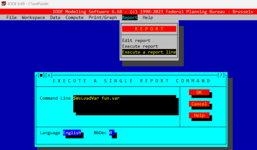
Old Interface: to execute an IODE command, you need to go to the menu Report and click on Execute a report line.

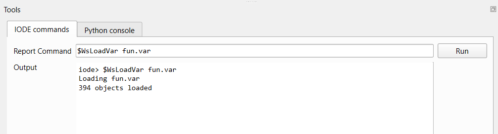
New Interface: to execute an IODE command, you need to open the IODE commands tab in the bottom panel, to type the command in the Report Command edit line and then click on the Run button or press Enter.

In Python, an IODE command can be executed using the execute_command() function. For example:

import iode as io
io.execute_command("$WsLoadVar fun.var")

For more details on IODE commands, see the sections Execution Commands and IODE Commands.

IODE functions

IODE functions allow to perform basic operations such as string or list of strings processing, text replacement, object counting, etc.
They start with the special character @ and follow the syntax @function_name(arg1, arg2, …) (e.g.: @take(2, ABCDE) will return AB).
The names of IODE functions are not case sensitive (e.g.: @take(2, ABCDE) and @TAKE(2, ABCDE) are equivalent).

For more details on IODE functions, see the section Functions.

Macros

Macros represent user defined variables that can be used to store values and reuse them later in the report (and sub-reports). They are defined with the $define command ($define macro_name value) and their values are accessed using the syntax %macro_name%.
The names of macros are case sensitive (e.g.: $define my_macro 10 and $define MY_MACRO 10 are two different macros).

Example:

$define FROM 1990Y1
$define TO   2000Y1
$define END  2010Y1

$EqsEstimate %FROM% %TO% ACAF
$ModelSimulate %TO% %END%

For more details on macros, see the section Macros.

LEC Expressions

It is possible to evaluate and use the results of LEC expressions inside a report.
Evaluable expressions are enclosed between { and }.
Since IODE works with time vectors, the period at which the LEC expression has to be calculated must be specify:
- $settime period: sets the current evaluation period $t$ to the period period,
- $incrtime step: increments the current evaluation period $t$ by step periods,
The current evaluation period $t$ is defined as an integer that represents the number of periods since the first period of the IODE Variables workspace.
Additionally, the format of the LEC expression result can be specified using the syntax {LEC@format} where format is one of the following:
- {LEC@99.9}: calculates the expression, with 4 digits including 1 decimal place
- {LEC@.9}: calculates the expression, with 1 decimal place,
- {LEC@T}: calculates the expression, and converts it to a year (1990Y1, …)
Rules for evaluating the expressions:
1. If a report line contains a {, then the text is read up to encountering a },
2. The macros present inside the expression are replaced by their values,
3. If the resulting expression begins with a $ or #, the rest of the expression is executed as a report command. The result (0 or 1) replaces the text in the report.
4. Otherwise, the expression is interpreted as a LEC formula and executed for the current evaluation period $t$ (determined by $settime). The (formatted) result replaces the text in the report.

Example:

$SetTime 1990Y1
$show The value of the current evaluation period t is {t}
$IncrTime 10
$show The incremented value of t is now {t@T}
$show Value of the coefficient acaf1 with two decimals: {acaf1@.99}
$show Successfully loaded Variables ? {$WsLoadVar fun.av}

Fore more details on LEC expressions, see the section LEC Expressions.

Comments

Lines starting with # or $ but followed by space are comments and do not execute and are print as it (e.g.: $WsLoadVar fun.var is a command line but $ WsLoadVar fun.var is a comment line).
Expressions between backquotes ` are also comments and are not executed (e.g.: the report line `@take(2, ABCDE) = ` @take(2,ABCDE) will print @take(2, ABCDE) = AB in the report output).

Report Arguments

Arguments passed to the reports are special macros and are accessed using the syntax %1% (first argument), %2% (second argument), etc.
The special variable %0% contains the number of passed arguments
The special variable %*% contains the list of all passed arguments.
The command $shift p shifts the arguments by p positions. The former %n% argument becomes %n-p% argument. Also %0% and %*% are updated.
Calling $shift without specifying p will shift arguments by 1 position.
After shifting, the shifted arguments disappear.

Error Handling

$onerror action specifies what should happen if something goes wrong in a report:
- ignore: (default) the report continues,
- return: the current (sub-)report stops,
- abort: all running reports stop,
- quit: exits the graphical user interface (GUI) and all running reports stop,
- display: (default) displays the error message on the screen,
- print: prints the error message,
- noprint: suppresses the error message
$debug {Yes|No}: displays the progress of the output
$abort: stops all running reports
$return: exits the current (sub-)report and continues with parent report
$quit: exits the graphical user interface (GUI) and all running reports stop

Feedback

$sleep nn: IODE sleeps for nn microseconds.
$show msg: IODE displays the message msg at the bottom of the screen. The report continues as usual.
$msg msg: IODE pauses the report and displays the message msg in a box dialog. The report stops until the user closes the box dialog.

Looping

The $foreach command allows you to specify an index and the list of values that this index should successively take.
The $next command returns to the start of the $foreach loop and moves to the next value of the index.

Syntax:

$indent
$foreach {index} {values}
  ...
  $next {index}

where:

{index} is a macro name of up to 10 characters (for example i, idx, COUNTRY, …)
{values} is a list of values separated by commas, spaces, or semicolons. The separators can be changed with the $vseps command.

Example 1: nested loops:

$indent
$foreach I BE BXL VL WAL
  $foreach J H F
    $show [%I%;%J%]
  $next J
$next I

Example 2: using lists:

$indent
$DataUpdateLst MYLIST X,Y,Z
$Define n 0
$foreach I @lvalue(MYLIST)
  $Define n {%n% + 1}
  $show Element %n% : [%I%]
  $next I

Jumping

$label name: places an anchor and gives it a name.
$goto name {condition}: execution of the report jumps to name. An optional condition can be specified.

Example:

$goto exist {$DataExistVar A}
$show Variable A does not exist
$return
$label exist
$show Variable A exists
$return

Warning

Be careful of infinite loop if the goto refers to a label defined above in the goto!

Note

In Python, there is no direct equivalent (goto like statement have been avoided in modern languages due to their potential to create complex and hard-to-maintain code). Use if-else statements and user defined functions to control the flow of your Python code instead.

Procedures

Procedures are groups of commands that can be defined and then called with different parameters. They are useful to avoid code duplication and to improve the maintenance of IODE reports.

Procedures are related to the commands $procdef, $procend, and $procexec.

Example:

$procdef procname [fparm1 ...]
  ...
$procend

where:

procname is the name of the procedure (case sensitive).
fparm1 is the first parameter of the procedure

A procedure is called simply with the command:

$procexec procname aparm1 ...

where:

procname is the name of the procedure (case sensitive).
aparm1 is the first passed parameter of the procedure

Scope of a procedure definition

Procedures must be defined before they can be called.
Once defined, a procedure remains callable within the same IODE session, even if the report that defined it has finished. You can execute a report whose sole purpose is to load procedures into memory. These procedures will remain available throughout the session.
A procedure can be replaced at any time by another with the same name.

For more details on procedures, see $procdef.

Computed Tables

One of the most frequently performed operations during a simulation exercise is the display of tables of results and charts. It may also be useful to compare the results of different simulations or to compare them with observed data. That is the purpose of the IODE tables.

An IODE table is computed according to a generalized sample and optional extra files (containing the results of previous simulations).

A generalized sample contains the following information:

the sampling of the periods to take into account
the operations to be performed on the periods
the list of files involved in the computation of the table
the operations to be performed between files
the repetition factor

The syntax of the generalized sample follows the rules described below.

Syntax for Periods

a period is indicated as in LEC: yyPpp or yyyyPpp where yyyy indicates the year, P the periodicity and pp the sub-period (e.g. 1990Y1)
a period can be shifted n periods to the left or right using the operators <n and >n
when used with a zero argument, the shift operators have a special meaning:
- <0 means “first period of the year”
- >0 means “last period of the year”
the special periods ‘BOS’, ‘EOS’ and ‘NOW’ can be used to represent the beginning or end of the current sample or the current period (PC clock)
the special periods ‘BOS1’, ‘EOS1’ and ‘NOW1’ are equivalent to the previous ones, except that they are moved to the first sub-period of the year of ‘BOS’, ‘EOS’ and ‘NOW’ respectively (if NOW = 2012M5, NOW1 = 2012M1)
each period is separated from the next by a semicolon
a period or group of periods can be repeated: simply place the colon character (:) after the definition of the column or group of columns, followed by the desired number of repetitions. Repetitions are made with an increment of one period, unless followed by an asterisk and a value. This value is then the repeat increment. It can be negative, in which case the periods are presented in decreasing order
the repeat, increment and shift can be the words PER (or P) or SUB (or S), which respectively indicate the number of periods in a year of the current sample and the current sub-period
the file definition is optional and is enclosed in square brackets. It applies to all preceding period definitions.

Operations on Periods

value: (75)
growth rate over one or more periods: (75/74, 75/70)
average growth rate: (75//70)
difference: (75-74, 75-70)
average difference: (75–70)
average: (75~74) or (75^74)
sum of consecutive periods: (70Q1+70Q4)
index or base value: (76=70)

Periods Repetition

Repetition can be performed with an increment greater than 1 or less than 0: simply place a star followed by the step after the number of repetitions (70:3*5 = 70, 75, 80).

Syntax for Files

absolute value: [1]
difference: [1-2]
difference in percent: [1/2]
sum: [1+2]
average: [1~2] or [1^2].

The file [1] always refers to the current workspace. Extra files (if passed as argument) are numerated from 2 to 5.

Examples

70; 75; 80:6 = 70:3*5; 81:5 = 70; 75; 80; 81; 82; 83; 84; 85
70/69:2 = 70/69; 71/70
(70; 70-69):2 = 70; 70-69; 71; 71-70;
70[1,2]:2*5 = 70[1]; 70[2]; 75[1]; 75[2]
(70;75)[1,2-1] = 70[1]; 75[1]; 70[2-1]; 75[2-1]
(70;75;(80; 80/79):2)[1,2] = 70[1]; 70[2]; 75[1]; 75[2]; 80[1]; 80[2]; 80/79[1]; 80/79[2] 81[1]; 8[2]; 8180[1]; 81/80[2]
2000Y1>5 = 2005Y1
1999M1>12 = 2000M1
EOS<1 = 2019Y1                         (if EOS == 2020Y1)
BOS<1 = 1959Y1                         (if BOS == 1960Y1)
EOS<4:5*-1 =2016;2017;2018;2019;2020   (if EOS = 2020Y1)

List of IODE Commands for Computed Tables

PrintTblFile: defines files to use when printing comparison tables
PrintTbl: builds and prints tables in A2M format
ViewTblFile: defines files to use when viewing comparison tables
ViewTbl: builds and displays tables in a scrollable table
ViewByTbl: alias for ViewTbl
PrintVar: builds and prints comparison tables of series in A2M format
ViewVar: views comparison tables of series in A2M format
ViewNdec: specifies the number of decimals for values displayed in tables
ViewGr: displays tables as graphs
PrintGr: prints one or more graphs defined from tables
DataPrintGraph: prints graphs built directly from variables

Tutorial

LEC language

What Is LEC?

Basic Building Blocks

Numeric constants

Language constants

Temporal constants and t

Variables and Scalars

Variables

Scalars

Time Indexing (Lag, Lead, Fixed Period)

Algebraic and Logical Operators

Mathematical Functions

Time Functions

Special Variable i in Sub-Expressions

Lists and Macros

Named lists

Computed lists with wildcards

Comments

Operator Precedence

Writing Equations

Quick Syntax Reminder

IODE reports

Purpose And Context

Running Reports

Graphical User Interface (GUI)

Command Line (Windows Terminal)

Python

Modular Report Invocation

IODE Commands

IODE functions

Macros

LEC Expressions

Comments

Report Arguments

Error Handling

Feedback

Looping

Jumping

Procedures

Scope of a procedure definition

Computed Tables

Syntax for Periods

Operations on Periods

Periods Repetition

Syntax for Files

Examples

List of IODE Commands for Computed Tables

Python Package

Special Variable `i` in Sub-Expressions