Getting Started
The purpose of the present Getting Started section is to give a quick overview of the main objects, methods and functions of the Python iode library. To get a more detailed presentation of all capabilities of iode, read the next sections of the tutorial.
The Installation section describes how to install the iode library and the iode-gui graphical user interface and their dependencies.
The Introduction section gives a brief overview of the concepts of the IODE tool.
The The LEC Language section describes the LEC language (”Langage Econométrique Condensé”), which is the scripting language used in the IODE tool to define equations, identities or any mathematical expressions to be evaluated.
The API Reference section of the documentation give you the list of all IODE commands and IODE functions with their individual documentation and examples.
The API Reference Python section of the documentation give you the list of all Python objects, methods and functions with their individual documentation and examples.
To use the Python iode library, the first thing to do is to import objects and functions you need from it:
[1]:
import numpy as np
import pandas as pd
import larray as la

from iode import SAMPLE_DATA_DIR, NA
To know the version of the iode library installed on your machine, type:
[2]:
from iode import __version__
__version__
[2]:
'7.0.6'
To print the documentation of an object, method or function in a Python interactive console, use the help() function:
[3]:
from iode import equations

# ---- print documentation of a function or method ----
help(equations.load)
Help on method load in module iode.iode_database.abstract_database:

load(filepath: str) method of iode.iode_database.equations_database.Equations instance
    Load objects stored in file 'filepath' into the current database.
    Erase the database before to load the file.

    Parameters
    ----------
    filepath: str
        path to the file to load

    Examples
    --------
    >>> from iode import comments, equations, identities, lists, tables, scalars, variables
    >>> from iode import SAMPLE_DATA_DIR
    >>> comments.load(f"{SAMPLE_DATA_DIR}/fun.cmt")         # doctest: +ELLIPSIS, +NORMALIZE_WHITESPACE
    Loading .../fun.cmt
    317 objects loaded

    >>> equations.load(f"{SAMPLE_DATA_DIR}/fun.eqs")        # doctest: +ELLIPSIS, +NORMALIZE_WHITESPACE
    Loading .../fun.eqs
    274 objects loaded

    >>> identities.load(f"{SAMPLE_DATA_DIR}/fun.idt")       # doctest: +ELLIPSIS, +NORMALIZE_WHITESPACE
    Loading .../fun.idt
    48 objects loaded

    >>> lists.load(f"{SAMPLE_DATA_DIR}/fun.lst")            # doctest: +ELLIPSIS, +NORMALIZE_WHITESPACE
    Loading .../fun.lst
    17 objects loaded

    >>> tables.load(f"{SAMPLE_DATA_DIR}/fun.tbl")           # doctest: +ELLIPSIS, +NORMALIZE_WHITESPACE
    Loading .../fun.tbl
    46 objects loaded

    >>> scalars.load(f"{SAMPLE_DATA_DIR}/fun.scl")          # doctest: +ELLIPSIS, +NORMALIZE_WHITESPACE
    Loading .../fun.scl
    161 objects loaded

    >>> variables.load(f"{SAMPLE_DATA_DIR}/fun.var")        # doctest: +ELLIPSIS, +NORMALIZE_WHITESPACE
    Loading .../fun.var
    394 objects loaded
IODE Objects
A model is a system of equations, which are formulas involving variables, numerical time series defined over a given period, with a specific frequency (annual, quarterly, etc.). The equations may contain coefficients (possibly estimated) which are dimensionless variables, called Scalars.
The variables themselves are not always obtained as such, but most often result from calculations based on other variables, possibly coming from several sources. These calculations can be, for example, sector aggregation or a geographic dimension. The formulas used to generate those variables are called identities.
The name given to each variable generally does not allow its content to be indicated with sufficient precision. IODE allows the creation of comments whose name will be identical to that of the variables they define. These comments are simply free text.
When variables are available, it is often useful to present them in the form of tables or charts. IODE allows the construction of special tables for this purpose. Those tables do not contain numerical values, but formulas and text. Then, these can be “computed” so as to obtain numerical tables (called computed tables) or charts. This approach is very efficient: the same table can be reused to print different versions of the variables (after simulating a scenario, for example). These tables can also be used to compare different scenarios or variants of a model by loading different files containing the same variables.
There is no notion of a model as an object in IODE: a model is simply a list of equations. To avoid the tedious work of re-encoding lists, these are managed as standalone objects and saved in list files. Lists are also used in formulas to shorten writing, or passed as parameters to IODE functions, etc.
Each object of one of the seven types is identified by a name of up to 20 characters. They always start with a letter or an underscore ‘_’. Their names are written in lowercase for scalars and in uppercase for other objects (so as to distinguish scalars and variables in LEC formulas).
Comment
IODE Comments are free text. They are used to document other IODE objects.
[4]:
cmt_ACAF = "Enterprises: received capital transfers"
cmt_ACAF
[4]:
'Enterprises: received capital transfers'
Equation
An equation represents an equality mixing variables and scalars (coefficients) and is part of a model. Each equation is composed of the following elements:
the LEC form (the formula scripting language in IODE)
a free comment (title of the Table)
the method by which it was estimated (if applicable)
the possible estimation period
the names of equations estimated simultaneously (block)
the instruments used for the estimation
All these definition elements are present in each equation, but may be left empty if not applicable.
The name of an equation is that of its endogenous variable. An equation can never be renamed, but it can be deleted and redefined with a new name.
To create an equation, you can use the constructor method of the Equation class:
[6]:
from iode import Equation, variables
# initialize the sample (range of periods) of the 'variables' workspace
variables.sample = "1960Y1:2015Y1"
# create a new equation
eq_ACAF = Equation("ACAF", "(ACAF / VAF[-1]) := acaf1 + acaf2 * GOSF[-1] + acaf4 * (TIME=1995)")
eq_ACAF
[6]:
Equation(endogenous = 'ACAF',
         lec = '(ACAF / VAF[-1]) := acaf1 + acaf2 * GOSF[-1] + acaf4 * (TIME=1995)',
         method = 'LSQ',
         from_period = '1960Y1',
         to_period = '2015Y1')
To access and modify the elements of an equation, you can use the following attributes:
[7]:
# endogenous variables of the equation
# (= equation's name)
eq_ACAF.endogenous
[7]:
'ACAF'
Warning: the endogenous variable of an equation is the name of the equation itself and cannot be changed:
[8]:
try:
    eq_ACAF.endogenous = "ACAF_"
except AttributeError as e:
    print(f"Error: {e}")
Error: property 'endogenous' of 'Equation' object has no setter
[9]:
# LEC form of the equation
eq_ACAF.lec
[9]:
'(ACAF / VAF[-1]) := acaf1 + acaf2 * GOSF[-1] + acaf4 * (TIME=1995)'
[10]:
eq_ACAF.lec = "ACAF / VAF[-1] := acaf1 + acaf2 * GOSF[-1] + acaf4 * (TIME=1995)"
eq_ACAF.lec
[10]:
'ACAF / VAF[-1] := acaf1 + acaf2 * GOSF[-1] + acaf4 * (TIME=1995)'
[11]:
# estimation method of the equation
eq_ACAF.method
[11]:
'LSQ'
[12]:
from iode import EqMethod
eq_ACAF.method = EqMethod.MAX_LIKELIHOOD
eq_ACAF.method
[12]:
'MAX_LIKELIHOOD'
[13]:
# range of periods for which the equation is estimated
# By default, it is the sample of the 'variables' workspace
eq_ACAF.sample
[13]:
Sample("1960Y1:2015Y1")
[14]:
eq_ACAF.sample = "1980Y1:1996Y1"
eq_ACAF.sample
[14]:
Sample("1980Y1:1996Y1")
[15]:
# block of equations to which the equation belongs
# A block of equations is a group of equations that are estimated together
eq_ACAF.block
[15]:
''
[16]:
eq_ACAF.block = "ACAF;DPUH"
eq_ACAF.block
[16]:
'ACAF;DPUH'
[17]:
# comment associated with the equation
eq_ACAF.comment
[17]:
''
[18]:
eq_ACAF.comment = cmt_ACAF
eq_ACAF.comment
[18]:
'Enterprises: received capital transfers'
[19]:
# instruments associated with the equation
eq_ACAF.instruments
[19]:
''
[20]:
eq_ACAF.instruments = ["GOSF", "VAF"]
eq_ACAF.instruments
[20]:
['GOSF', 'VAF']
[21]:
# tests evaluated during the estimation of the equation
eq_ACAF.tests
[21]:
{'corr': 0.0,
 'dw': 0.0,
 'fstat': 0.0,
 'loglik': 0.0,
 'meany': 0.0,
 'r2': 0.0,
 'r2adj': 0.0,
 'ssres': 0.0,
 'stderr': 0.0,
 'stderrp': 0.0,
 'stdev': 0.0}
Warning: the tests associated with an equation are set during the estimation process and cannot be modified manually.
[22]:
try:
    eq_ACAF.tests = [1.0, 2.32935, 32.2732, 83.8075, 0.00818467, 0.821761, 0.796299,
                     5.19945e-05, 0.00192715, 23.5458, 0.0042699]
except AttributeError as e:
    print(f"Error: {e}")
Error: property 'tests' of 'Equation' object has no setter
Warning: in the same way, the date attribute of an equation is updated during the estimation process and cannot be modified manually.
[23]:
# last date of estimation of the equation
eq_ACAF.date
[23]:
''
[24]:
try:
    eq_ACAF.date = "04-06-2025"
except AttributeError as e:
    print(f"Error: {e}")
Error: property 'date' of 'Equation' object has no setter
To get the list of scalars (coefficients) and variables referenced in an Equation, use the coefficients and variables properties of the Equation class:
[25]:
eq_ACAF.coefficients
[25]:
['acaf1', 'acaf2', 'acaf4']
[26]:
eq_ACAF.variables
[26]:
['ACAF', 'VAF', 'GOSF', 'TIME']
To split an equation into its left-hand side and its right-hand side, use the split_equation method of the Equation class:
[27]:
left, right = eq_ACAF.split_equation()
print("left-hand side: ", left)
print("right-hand side:", right)
left-hand side:  ACAF / VAF[-1]
right-hand side: acaf1 + acaf2 * GOSF[-1] + acaf4 * (TIME=1995)
To estimate the an equation, use the estimate method of the Equation class.
At the end of the estimation process, certain variables and scalars are automatically created if the process has converged. These variables and scalars can be used for computational purposes and, as they are part of the global workspace, can be saved for future use.
The tests resulting from the last estimation are saved as scalars. The same applies to residuals, left-hand and right-hand members of equations.
Saved tests (as scalars) have the following names:
e0_n: number of sample periodse0_k: number of estimated coefficientse0_stdev: std dev of residualse0_meany: mean of Ye0_ssres: sum of squares of residualse0_stderr: std errore0_stderrp: std error percent (in %)e0_fstat: F-State0_r2: R squaree0_r2adj: adjusted R-squarede0_dw: Durbin-Watsone0_loglik: Log Likelihood
Calculated series are saved in special variables:
_YCALC0: right-hand side of the equation_YOBS0: left-hand side of the equation_YRES0: residuals of the equation
Outside the estimation sample, the series values are NA (Not Available):
[28]:
success = eq_ACAF.estimate("1980Y1", "2000Y1")
success
Estimating : iteration 1 (||eps|| = 0.0566493)
Estimating : iteration 2 (||eps|| = 0.0594508)
Estimating : iteration 3 (||eps|| = 0.0117815)
Estimating : iteration 4 (||eps|| = 0.00240163)
Estimating : iteration 5 (||eps|| = 0.000492758)
Estimating : iteration 6 (||eps|| = 0.000101281)
Estimating : iteration 7 (||eps|| = 2.08105e-05)
Estimating : iteration 8 (||eps|| = 4.27624e-06)
Estimating : iteration 9 (||eps|| = 8.78712e-07)
Solution reached after 9 iteration(s). Creating results file ...
[28]:
True
[29]:
eq_ACAF.tests
[29]:
{'corr': 1.0,
 'dw': 1.8939709663391113,
 'fstat': 34.6290397644043,
 'loglik': 158.13970947265625,
 'meany': 0.007528899237513542,
 'r2': 0.7937153577804565,
 'r2adj': 0.7707948684692383,
 'ssres': 7.38456001272425e-05,
 'stderr': 0.002025471068918705,
 'stderrp': 26.902618408203125,
 'stdev': 0.004230715800076723}
[30]:
eq_ACAF.date
[30]:
'19-03-2026'
Identity
An identity is an expression written in the LEC language that allows the construction of a new statistical series based on already defined series. In general, identities are executed in groups to create or update a set of variables. Identities can be executed for a specific range of periods, or for all periods defined in the workspace.
Identities should not be confused with equations. They are not part of a model.
To create an identity, you can use the constructor method of the Identity class:
[31]:
from iode import Identity
idt = Identity("1 - exp((gamma2 + gamma3 * ln(W/ZJ)[-1] + gamma4 * ln(WMIN/ZJ)) / gamma_)")
idt
[31]:
Identity('1 - exp((gamma2 + gamma3 * ln(W/ZJ)[-1] + gamma4 * ln(WMIN/ZJ)) / gamma_)')
To get the list of scalars (coefficients) and variables referenced in an identity, use the coefficients and variables properties of the Identity class:
[32]:
idt.coefficients
[32]:
['gamma2', 'gamma3', 'gamma4', 'gamma_']
[33]:
idt.variables
[33]:
['W', 'ZJ', 'WMIN']
List
IODE Lists are either free text (like IODE comments) or a Python list. They are used to simplify writing in various circumstances:
list of equations defining a model
list of tables to print
any argument of a function (such as print period)
macro in an equation, identity, or table
etc.
[34]:
A_VARS = ["ACAF", "ACAG", "AOUC", "AOUC_", "AQC"]
A_VARS
[34]:
['ACAF', 'ACAG', 'AOUC', 'AOUC_', 'AQC']
Scalar
Scalars are essentially estimated coefficients of econometric equations. For this reason, each scalar contains in its definition:
its value
the relaxation parameter, set to 0 to lock the coefficient during estimation
its standard deviation, result of the last estimation
Only the values of the scalars are relevant when calculating a LEC expression. The other two values (relaxation and standard deviation) are only meaningful for estimation.
The names of scalars must be in lowercase so that variables are distinct from scalars in LEC formulas.
To create a scalar, you can use the constructor method of the Scalar class:
[35]:
import numpy as np
from iode import Scalar

# default relax
scalar = Scalar(0.9)
scalar
[35]:
Scalar(0.9, 1, na)
[36]:
# specific value and relax
scalar = Scalar(0.9, 0.8)
scalar
[36]:
Scalar(0.9, 0.8, na)
[37]:
# Python nan are converted to IODE NA
scalar = Scalar(np.nan)
scalar
[37]:
Scalar(na, 1, na)
[38]:
# Python inf are not accepted
try:
    scalar = Scalar(np.inf)
except ValueError as e:
    print(f"Error: {e}")
Error: Expected 'value' to be a finite number
[39]:
# relax must be between 0.0 and 1.0
try:
    scalar = Scalar(0.9, 1.1)
except ValueError as e:
    print(f"Error: {e}")
Error: Expected 'relax' value between 0.0 and 1.0
To access and modify the value and relax of a scalar, use the following attributes:
[40]:
scalar.value
[40]:
nan
[41]:
scalar.value = 0.95
scalar.value
[41]:
0.95
[42]:
scalar.relax
[42]:
1.0
[43]:
scalar.relax = 0.85
scalar.relax
[43]:
0.85
To access standard deviation of a scalar, use the std attribute:
[44]:
scalar.std
[44]:
nan
Warning: the standard deviation of a scalar is set during the estimation process and cannot be modified manually.
[45]:
try:
    scalar.std = 0.001369
except AttributeError as e:
    print(f"Error: {e}")
Error: property 'std' of 'Scalar' object has no setter
Table
One of the most frequently performed operations during a simulation exercise is the display of tables of results and charts.
Each IODE table is a set of lines. A line is composed of two parts (in general):
a text part, which will be the title of the line
a formula part, which will allow the calculation of the numerical values to be placed in the computed table:
TABLE TITLE
Gross National Product GNPUnemployment ULExternal Balance X-I
The lines are actually of several types:
TITLE lines (centered on the page width),
CELL lines (title + formula),
SEPARATOR lines
MODE lines
FILES lines
DATE lines
A table is designed to be “computed” over different periods, described by a “generalized sample” such as:
1980Y1:10 –> 10 observations from 1980Y1 1980Y1, 1985Y1, 1990:5 –> 1980, 1985, then 5 observations from 1990Y1 80/79:5 –> 5 growth rates from 1980 …
It can also contain values from different files:
(1990:5)[1,2,1-2] –> values from 1990 to 1994 for files 1, 2, and for the difference between the two files.
The computed table can be:
displayed on screen
printed
exported as a chart
exported to a file (in CSV, HTML, …)
(Python) converted to a Pandas DataFrame or an larray Array
Tables can very well be used in a project that does not include an econometric model: the only information used by tables are variables and possibly scalars.
Create A Table
To create an IODE table, you can either:
Call the Table constructor without any argument. This will create an empty table with two columns. Then you can add lines using the += operator or the insert() method (see next section).
[46]:
from iode import Table

# empty table
table = Table()
table
[46]:
DIVIS | 1 |
TITLE |
----- | --------
CELL  |   | "#S"
----- | --------

nb lines: 4
nb columns: 2
language: 'ENGLISH'
gridx: 'MAJOR'
gridy: 'MAJOR'
graph_axis: 'VALUES'
graph_alignment: 'LEFT'
Call the Table constructor with a title and a list of variables. This list can contain IODE list(s) referenced with a
$symbol. In that case, the IODE list(s) will be expanded to its (their) content. For each row, if an IODE comment with the same name as the variable exists, the value of the comment will be used in the left column. If the comment does not exist, the name of the variable will be used. The boolean arguments mode, files and date can be used to append the corresponding special lines to the table. These three lines are used when the table is computed (according to a generalized sample):
[47]:
# content of the IODE list 'ENVI'
lists["ENVI"]
[47]:
['EX',
 'PWMAB',
 'PWMS',
 'PWXAB',
 'PWXS',
 'QWXAB',
 'QWXS',
 'POIL',
 'NATY',
 'TFPFHP_']
[48]:
# create a table using a list of variables
# NOTE: the list of variables can contain IODE list(s).
#       The IODE list(s) must be referenced using the '$' symbol
table_title = "Table example with variables only"
lines_vars = ["GOSG", "YDTG", "DTH", "DTF", "IT", "YSSG", "COTRES", "RIDG", "OCUG", "$ENVI"]
table = Table(2, table_title, lines_vars, mode=True, files=True, date=True)
table
[48]:
DIVIS | 1                                                                    |
TITLE |                      "Table example with variables only"
----- | ------------------------------------------------------------------------------
CELL  |                                                                      |   "#S"
----- | ------------------------------------------------------------------------------
CELL  | "Bruto exploitatie-overschot: overheid (= afschrijvingen)."          |    GOSG
CELL  | "Overheid: geïnde indirecte belastingen."                            |    YDTG
CELL  | "Totale overheid: directe belasting van de gezinnen."                |     DTH
CELL  | "Totale overheid: directe vennootschapsbelasting."                   |     DTF
CELL  | "Totale indirecte belastingen."                                      |      IT
CELL  | "Globale overheid: ontvangen sociale zekerheidsbijdragen."           |    YSSG
CELL  | "Cotisation de responsabilisation."                                  |  COTRES
CELL  | "Overheid: inkomen uit vermogen."                                    |    RIDG
CELL  | "Globale overheid: saldo van de ontvangen lopendeoverdrachten."      |    OCUG
CELL  | "Wisselkoers van de USD t.o.v. de BEF (jaargemiddelde)."             |      EX
CELL  | "Index wereldprijs - invoer van niet-energieprodukten, inUSD."       |   PWMAB
CELL  | "Index wereldprijs - invoer van diensten, in USD."                   |    PWMS
CELL  | "Index wereldprijs - uitvoer van niet-energieprodukten, inUSD."      |   PWXAB
CELL  | "Index wereldprijs - uitvoer van diensten, in USD."                  |    PWXS
CELL  | "Indicator van het volume van de wereldvraag naar goederen,1985=1."  |   QWXAB
CELL  | "Indicator van het volume van de wereldvraag naar diensten,1985=1."  |    QWXS
CELL  | "Brent olieprijs (USD per barrel)."                                  |    POIL
CELL  | "Totale beroepsbevolking (jaargemiddelde)."                          |    NATY
CELL  | "TFPFHP_"                                                            | TFPFHP_
----- | ------------------------------------------------------------------------------
MODE  |
FILES |
DATE  |

nb lines: 27
nb columns: 2
language: 'ENGLISH'
gridx: 'MAJOR'
gridy: 'MAJOR'
graph_axis: 'VALUES'
graph_alignment: 'LEFT'
[49]:
# variables or LEC expressions can be also passed as a single string
lines_vars = "GOSG;YDTG;DTH;DTF;IT;YSSG;COTRES;RIDG;OCUG;$ENVI"
table_title = "Table example with all variables passed as a single string"
table = Table(2, table_title, lines_vars, mode=True, files=True, date=True)
table
[49]:
DIVIS | 1                                                                    |
TITLE |          "Table example with all variables passed as a single string"
----- | ------------------------------------------------------------------------------
CELL  |                                                                      |   "#S"
----- | ------------------------------------------------------------------------------
CELL  | "Bruto exploitatie-overschot: overheid (= afschrijvingen)."          |    GOSG
CELL  | "Overheid: geïnde indirecte belastingen."                            |    YDTG
CELL  | "Totale overheid: directe belasting van de gezinnen."                |     DTH
CELL  | "Totale overheid: directe vennootschapsbelasting."                   |     DTF
CELL  | "Totale indirecte belastingen."                                      |      IT
CELL  | "Globale overheid: ontvangen sociale zekerheidsbijdragen."           |    YSSG
CELL  | "Cotisation de responsabilisation."                                  |  COTRES
CELL  | "Overheid: inkomen uit vermogen."                                    |    RIDG
CELL  | "Globale overheid: saldo van de ontvangen lopendeoverdrachten."      |    OCUG
CELL  | "Wisselkoers van de USD t.o.v. de BEF (jaargemiddelde)."             |      EX
CELL  | "Index wereldprijs - invoer van niet-energieprodukten, inUSD."       |   PWMAB
CELL  | "Index wereldprijs - invoer van diensten, in USD."                   |    PWMS
CELL  | "Index wereldprijs - uitvoer van niet-energieprodukten, inUSD."      |   PWXAB
CELL  | "Index wereldprijs - uitvoer van diensten, in USD."                  |    PWXS
CELL  | "Indicator van het volume van de wereldvraag naar goederen,1985=1."  |   QWXAB
CELL  | "Indicator van het volume van de wereldvraag naar diensten,1985=1."  |    QWXS
CELL  | "Brent olieprijs (USD per barrel)."                                  |    POIL
CELL  | "Totale beroepsbevolking (jaargemiddelde)."                          |    NATY
CELL  | "TFPFHP_"                                                            | TFPFHP_
----- | ------------------------------------------------------------------------------
MODE  |
FILES |
DATE  |

nb lines: 27
nb columns: 2
language: 'ENGLISH'
gridx: 'MAJOR'
gridy: 'MAJOR'
graph_axis: 'VALUES'
graph_alignment: 'LEFT'
Call the Table constructor with a title, a list of line titles (left column) and a list of the variables names or LEC expressions (right column):
[50]:
table_title = "Table example with titles on the left and LEC expressions on the right"
# left column
lines_titles = ["GOSG:", "YDTG:", "DTH:", "DTF:", "IT:", "YSSG+COTRES:", "RIDG:", "OCUG:"]
# right column
lines_lecs = ["GOSG", "YDTG", "DTH", "DTF", "IT", "YSSG+COTRES", "RIDG", "OCUG"]
table = Table(2, table_title, lines_lecs, lines_titles, True, True, True)
table
[50]:
DIVIS | 1              |
TITLE | "Table example with titles on the left and LEC expressions on the right"
----- | ------------------------------------------------------------------------
CELL  |                |     "#S"
----- | ------------------------------------------------------------------------
CELL  | "GOSG:"        |        GOSG
CELL  | "YDTG:"        |        YDTG
CELL  | "DTH:"         |         DTH
CELL  | "DTF:"         |         DTF
CELL  | "IT:"          |          IT
CELL  | "YSSG+COTRES:" | YSSG+COTRES
CELL  | "RIDG:"        |        RIDG
CELL  | "OCUG:"        |        OCUG
----- | ------------------------------------------------------------------------
MODE  |
FILES |
DATE  |

nb lines: 16
nb columns: 2
language: 'ENGLISH'
gridx: 'MAJOR'
gridy: 'MAJOR'
graph_axis: 'VALUES'
graph_alignment: 'LEFT'
Get/Update The Divider Line
To update the divider line, use the divider attribute:
[51]:
# the default divider is 1
table.divider
[51]:
('1', '')
[52]:
# update the divider to multiply all values of the
# right column by 100 (e.g. to get percentage values)
table.divider = ('1', '1e-2')
table.divider
[52]:
('1', '1e-2')
Find The Position Of A Line
To find the position of a line in an IODE table, use the index(str) method:
[53]:
# find the index of the TITLE or CELL line containing RIDG
index = table.index("RIDG")
index
[53]:
10
Get/Update Content Of Lines
To get or update the content of a line, use the [index] operator:
[54]:
table[4]
[54]:
('"GOSG:"', 'GOSG')
Negative indices can be used to get or update the content of a line from the end of the table:
[55]:
# content of the last line
table[-1]
[55]:
<DATE>
Append Lines
To append a line to an IODE table, use the += operator:
[56]:
from iode import TableLineType

table = Table()

# append a title line
table += "Dummy Table"

# append a separator line
table += '-'

# append a line with cells
# NOTE: line containing double quotes " -> assumed to be a STRING cell
#       line without double quotes      -> assumed to be a LEC cell
table += ('"RIDG:"', 'RIDG')

# append a separator line (other way to do it)
table += TableLineType.SEP

# append a special MODE line
table += TableLineType.MODE

# append a special FILES line
table += TableLineType.FILES

# append a special DATE line
table += TableLineType.DATE

table
[56]:
DIVIS | 1       |
TITLE |
----- | --------------
CELL  |         | "#S"
----- | --------------
TITLE | "Dummy Table"
----- | --------------
CELL  | "RIDG:" | RIDG
----- | --------------
MODE  |
FILES |
DATE  |

nb lines: 11
nb columns: 2
language: 'ENGLISH'
gridx: 'MAJOR'
gridy: 'MAJOR'
graph_axis: 'VALUES'
graph_alignment: 'LEFT'
Insert Lines
To insert a line at a specific index, use the insert(index, value) method:
[57]:
# insert a CELL line before the RIDG line
index = table.index("RIDG")
table.insert(index, ('"OCUG:"', 'OCUG'))

# insert a CELL line after the RIDG line
index = table.index("RIDG")
table.insert(index + 1, ('"GOSG:"', 'GOSG'))

# insert a separator after the GOSG line
index = table.index("GOSG")
index += 1
table.insert(index, '-')

# insert a title line after the separator line
index += 1
table.insert(index, "New Title")

# insert a separator line after the title line
index += 1
table.insert(index, TableLineType.SEP)

table
[57]:
DIVIS | 1       |
TITLE |
----- | --------------
CELL  |         | "#S"
----- | --------------
TITLE | "Dummy Table"
----- | --------------
CELL  | "OCUG:" | OCUG
CELL  | "RIDG:" | RIDG
CELL  | "GOSG:" | GOSG
----- | --------------
TITLE |  "New Title"
----- | --------------
----- | --------------
MODE  |
FILES |
DATE  |

nb lines: 16
nb columns: 2
language: 'ENGLISH'
gridx: 'MAJOR'
gridy: 'MAJOR'
graph_axis: 'VALUES'
graph_alignment: 'LEFT'
Delete Lines
To delete a line, use the del keyword:
[58]:
index = table.index("New Title")

# delete the title line
del table[index]

table
[58]:
DIVIS | 1       |
TITLE |
----- | --------------
CELL  |         | "#S"
----- | --------------
TITLE | "Dummy Table"
----- | --------------
CELL  | "OCUG:" | OCUG
CELL  | "RIDG:" | RIDG
CELL  | "GOSG:" | GOSG
----- | --------------
----- | --------------
----- | --------------
MODE  |
FILES |
DATE  |

nb lines: 15
nb columns: 2
language: 'ENGLISH'
gridx: 'MAJOR'
gridy: 'MAJOR'
graph_axis: 'VALUES'
graph_alignment: 'LEFT'
Negative indices can be used to delete lines from the end of the table:
[59]:
# delete the last line
del table[-1]

table
[59]:
DIVIS | 1       |
TITLE |
----- | --------------
CELL  |         | "#S"
----- | --------------
TITLE | "Dummy Table"
----- | --------------
CELL  | "OCUG:" | OCUG
CELL  | "RIDG:" | RIDG
CELL  | "GOSG:" | GOSG
----- | --------------
----- | --------------
----- | --------------
MODE  |
FILES |

nb lines: 14
nb columns: 2
language: 'ENGLISH'
gridx: 'MAJOR'
gridy: 'MAJOR'
graph_axis: 'VALUES'
graph_alignment: 'LEFT'
Get the coefficients and variables of a table
To get the list of scalars (coefficients) and variables referenced in a table, use the coefficients and variables properties of the Table class:
[60]:
table.coefficients
[60]:
[]
[61]:
table.variables
[61]:
['GOSG', 'OCUG', 'RIDG']
Plotting
To plot a table, use the plot method:
[62]:
# variables or LEC expressions can be also passed as a single string
table_title = "Table for plotting"
# left column
lines_titles = ["GOSG", "YDTG", "DTH", "DTF", "IT", "YSSG+COTRES", "RIDG", "OCUG"]
# right column
lines_lecs = ["GOSG", "YDTG", "DTH", "DTF", "IT", "YSSG+COTRES", "RIDG", "OCUG"]
table = Table(2, table_title, lines_lecs, lines_titles, True, True, True)
table
[62]:
DIVIS | 1                                                           |
TITLE |                            "Table for plotting"
----- | -------------------------------------------------------------------------
CELL  |                                                             |     "#S"
----- | -------------------------------------------------------------------------
CELL  | "GOSG"                                                      |        GOSG
CELL  | "Bruto exploitatie-overschot: overheid (= afschrijvingen)." |        YDTG
CELL  | "DTH"                                                       |         DTH
CELL  | "Totale overheid: directe belasting van de gezinnen."       |         DTF
CELL  | "IT"                                                        |          IT
CELL  | "Totale indirecte belastingen."                             | YSSG+COTRES
CELL  | "RIDG"                                                      |        RIDG
CELL  | "Overheid: inkomen uit vermogen."                           |        OCUG
----- | -------------------------------------------------------------------------
MODE  |
FILES |
DATE  |

nb lines: 16
nb columns: 2
language: 'ENGLISH'
gridx: 'MAJOR'
gridy: 'MAJOR'
graph_axis: 'VALUES'
graph_alignment: 'LEFT'
[63]:
table.plot()
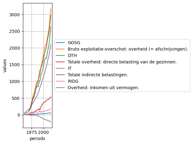
[63]:
<Axes: xlabel='periods', ylabel='values'>
Variable
Variables are series of numbers.
All variables from the “variables” workspace are defined over the same range of periods (sample). If observations are missing, they take the special value NA (Not Available) (displayed as -- in the graphical user interface).
Their names must be in uppercase so that variables are distinct from scalars in LEC formulas.
There is no Variable class in the Python iode library. Instead, a variable is represented by a subset of the variables workspace with one unique variable
Computed Tables
To compute a table according to a generalized sample and extra files, use the Table.compute method of the IODE table objects:
Calling compute(generalized_sample, extra_files, nb_decimals, quiet) computes the values corresponding to LEC expressions in cells.
The values are calculated for given a generalized sample. This sample contains the following information:
the sampling of the periods to take into account
the operations to be performed on the periods
the list of files involved in the computation of the table
the operations to be performed between files
the repetition factor
The syntax of the generalized sample follows the rules described below. The syntax of a period:
a period is indicated as in LEC:
yyPpporyyyyPppwhere yyyy indicates the year, P the periodicity and pp the sub-period (e.g. 1990Y1)a period can be shifted n periods to the left or right using the operators
<nand>nwhen used with a zero argument, the shift operators have a special meaning:
<0means “first period of the year”>0means “last period of the year”
the special periods ‘BOS’, ‘EOS’ and ‘NOW’ can be used to represent the beginning or end of the current sample or the current period (PC clock)
the special periods ‘BOS1’, ‘EOS1’ and ‘NOW1’ are equivalent to the previous ones, except that they are moved to the first sub-period of the year of ‘BOS’, ‘EOS’ and ‘NOW’ respectively (if NOW = 2012M5, NOW1 = 2012M1)
each period is separated from the next by a semicolon
a period or group of periods can be repeated: simply place the colon character (
:) after the definition of the column or group of columns, followed by the desired number of repetitions. Repetitions are made with an increment of one period, unless followed by an asterisk and a value. This value is then the repeat increment. It can be negative, in which case the periods are presented in decreasing orderthe repeat, increment and shift can be the words PER (or P) or SUB (or S), which respectively indicate the number of periods in a year of the current sample and the current sub-period
the file definition is optional and is enclosed in square brackets. It applies to all preceding period definitions.
The following file operations are possible:
absolute value: [1]
difference: [1-2]
difference in percent: [1/2]
sum: [1+2]
average: [1~2] or [1^2].
The file [1] always refers to the current workspace. Extra files (if passed as argument) are numerated from 2 to 5. The following period operations are possible:
value: (75)
growth rate over one or more periods: (75/74, 75/70)
average growth rate: (75//70)
difference: (75-74, 75-70)
average difference: (75–70)
average: (75~74) or (75^74)
sum of consecutive periods: (70Q1+70Q4)
index or base value: (76=70)
Repetition can be performed with an increment greater than 1 or less than 0: simply place a star followed by the step after the number of repetitions (70:3*5 = 70, 75, 80).
Generalized sample examples:
70; 75; 80:6 = 70:3*5; 81:5 = 70; 75; 80; 81; 82; 83; 84; 85
70/69:2 = 70/69; 71/70
(70; 70-69):2 = 70; 70-69; 71; 71-70;
70[1,2]:2*5 = 70[1]; 70[2]; 75[1]; 75[2]
(70;75)[1,2-1] = 70[1]; 75[1]; 70[2-1]; 75[2-1]
(70;75;(80; 80/79):2)[1,2] = 70[1]; 70[2]; 75[1]; 75[2]; 80[1]; 80[2]; 80/79[1]; 80/79[2] 81[1]; 8[2]; 8180[1]; 81/80[2]
2000Y1>5 = 2005Y1
1999M1>12 = 2000M1
EOS<1 = 2019Y1                         (if EOS == 2020Y1)
BOS<1 = 1959Y1                         (if BOS == 1960Y1)
EOS<4:5*-1 =2016;2017;2018;2019;2020   (if EOS = 2020Y1)
Examples
[64]:
table_title = "Table example with titles on the left and LEC expressions on the right"
# left column
lines_titles = ["GOSG:", "YDTG:", "DTH:", "DTF:", "IT:", "YSSG+COTRES:", "RIDG:", "OCUG:"]
# right column
lines_lecs = ["GOSG", "YDTG", "DTH", "DTF", "IT", "YSSG+COTRES", "RIDG", "OCUG"]
table = Table(2, table_title, lines_lecs, lines_titles, True, True, True)
table
[64]:
DIVIS | 1              |
TITLE | "Table example with titles on the left and LEC expressions on the right"
----- | ------------------------------------------------------------------------
CELL  |                |     "#S"
----- | ------------------------------------------------------------------------
CELL  | "GOSG:"        |        GOSG
CELL  | "YDTG:"        |        YDTG
CELL  | "DTH:"         |         DTH
CELL  | "DTF:"         |         DTF
CELL  | "IT:"          |          IT
CELL  | "YSSG+COTRES:" | YSSG+COTRES
CELL  | "RIDG:"        |        RIDG
CELL  | "OCUG:"        |        OCUG
----- | ------------------------------------------------------------------------
MODE  |
FILES |
DATE  |

nb lines: 16
nb columns: 2
language: 'ENGLISH'
gridx: 'MAJOR'
gridy: 'MAJOR'
graph_axis: 'VALUES'
graph_alignment: 'LEFT'
[65]:
# simple time series (current workspace) - 6 observations - 4 decimals
computed_table = table.compute("2000:6", nb_decimals=4)
computed_table
[65]:
 line title \ period[file]  |    2000   |    2001   |    2002   |    2003   |    2004   |    2005
----------------------------------------------------------------------------------------------------
GOSG:                       |   32.7013 |   34.5183 |   35.9341 |   37.3602 |   39.0778 |   40.6990
YDTG:                       | 1841.7930 | 1913.4770 | 1999.8462 | 2042.4147 | 2097.7328 | 2094.7998
DTH:                        | 1477.3851 | 1539.1702 | 1614.1974 | 1661.0073 | 1697.6353 | 1690.1593
DTF:                        |  364.4079 |  374.3072 |  385.6475 |  381.4071 |  400.0916 |  404.6382
IT:                         | 1146.7131 | 1202.9021 | 1242.0110 | 1288.0103 | 1342.8635 | 1401.3764
YSSG+COTRES:                | 1680.2238 | 1752.5931 | 1818.5073 | 1891.1969 | 1932.6684 | 1970.2945
RIDG:                       |   98.7683 |  104.2563 |  108.5322 |  112.8396 |  118.0272 |  122.9238
OCUG:                       | -120.7692 | -127.4797 | -132.7081 | -137.9749 | -144.3181 | -150.3054
[66]:
# get lines of the computed table
computed_table.lines
[66]:
['GOSG:', 'YDTG:', 'DTH:', 'DTF:', 'IT:', 'YSSG+COTRES:', 'RIDG:', 'OCUG:']
[67]:
# get columns of the computed table
computed_table.columns
[67]:
['2000', '2001', '2002', '2003', '2004', '2005']
[68]:
# two time series (current workspace) - 5 observations - 2 decimals (default)
computed_table = table.compute("(2010;2010/2009):5")
computed_table
[68]:
 line title \ period[file]  |   2010  | 2010/2009 |   2011  | 2011/2010 |   2012  | 2012/2011 |   2013  | 2013/2012 |   2014  | 2014/2013
------------------------------------------------------------------------------------------------------------------------------------------
GOSG:                       |   47.36 |      2.40 |   48.81 |      3.07 |   50.73 |      3.94 |   53.07 |      4.62 |   55.74 |      5.02
YDTG:                       | 2456.29 |      3.16 | 2554.61 |      4.00 | 2681.32 |      4.96 | 2832.01 |      5.62 | 2998.33 |      5.87
DTH:                        | 1999.96 |      3.38 | 2083.70 |      4.19 | 2193.41 |      5.26 | 2326.45 |      6.07 | 2477.09 |      6.47
DTF:                        |  456.33 |      2.17 |  470.90 |      3.19 |  487.91 |      3.61 |  505.56 |      3.62 |  521.24 |      3.10
IT:                         | 1688.71 |      2.49 | 1752.86 |      3.80 | 1830.30 |      4.42 | 1918.71 |      4.83 | 2012.81 |      4.90
YSSG+COTRES:                | 2370.44 |      2.94 | 2448.77 |      3.30 | 2551.46 |      4.19 | 2680.09 |      5.04 | 2824.22 |      5.38
RIDG:                       |  143.04 |      2.40 |  147.42 |      3.07 |  153.22 |      3.94 |  160.30 |      4.62 |  168.34 |      5.02
OCUG:                       | -174.90 |      2.40 | -180.26 |      3.07 | -187.36 |      3.94 | -196.01 |      4.62 | -205.84 |      5.02
[69]:
from pathlib import Path

# simple time series (current workspace + one extra file) - 5 observations - 2 decimals (default)
sample_data_dir = Path(SAMPLE_DATA_DIR)
computed_table = table.compute("2010[1;2]:5", extra_files=sample_data_dir/"ref.av", quiet=True)
computed_table
[69]:
 line title \ period[file]  | 2010[1] | 2010[2] | 2011[1] | 2011[2] | 2012[1] | 2012[2] | 2013[1] | 2013[2] | 2014[1] | 2014[2]
--------------------------------------------------------------------------------------------------------------------------------
GOSG:                       |   47.36 |   47.36 |   48.81 |   48.81 |   50.73 |   50.73 |   53.07 |   53.07 |   55.74 |   55.74
YDTG:                       | 2456.29 | 2456.29 | 2554.61 | 2554.61 | 2681.32 | 2681.32 | 2832.01 | 2832.01 | 2998.33 | 2998.33
DTH:                        | 1999.96 | 1999.96 | 2083.70 | 2083.70 | 2193.41 | 2193.41 | 2326.45 | 2326.45 | 2477.09 | 2477.09
DTF:                        |  456.33 |  456.33 |  470.90 |  470.90 |  487.91 |  487.91 |  505.56 |  505.56 |  521.24 |  521.24
IT:                         | 1688.71 | 1688.71 | 1752.86 | 1752.86 | 1830.30 | 1830.30 | 1918.71 | 1918.71 | 2012.81 | 2012.81
YSSG+COTRES:                | 2370.44 | 2370.44 | 2448.77 | 2448.77 | 2551.46 | 2551.46 | 2680.09 | 2680.09 | 2824.22 | 2824.22
RIDG:                       |  143.04 |  143.04 |  147.42 |  147.42 |  153.22 |  153.22 |  160.30 |  160.30 |  168.34 |  168.34
OCUG:                       | -174.90 | -174.90 | -180.26 | -180.26 | -187.36 | -187.36 | -196.01 | -196.01 | -205.84 | -205.84
[70]:
# get the list of files used to compute the table
# (the first file represents the current workspace)
computed_table.files
[70]:
['c:\\soft\\miniconda3\\Lib\\site-packages\\iode\\tests\\data\\fun.var',
 'C:\\soft\\miniconda3\\Lib\\site-packages\\iode\\tests\\data\\ref.av']
[71]:
# simple time series (current workspace + 4 extra files) - 5 observations - 2 decimals (default)
extra_files = [sample_data_dir / "ref.av", sample_data_dir / "fun.av",
               sample_data_dir / "fun2.av", sample_data_dir / "a.var"]
computed_table = table.compute("2010[1;2;3;4;5]:1", extra_files=extra_files, quiet=True)
computed_table
[71]:
 line title \ period[file]  | 2010[1] | 2010[2] | 2010[3] | 2010[4] | 2010[5]
------------------------------------------------------------------------------
GOSG:                       |   47.36 |   47.36 |   47.36 |   47.36 |      --
YDTG:                       | 2456.29 | 2456.29 | 2456.29 | 2456.29 |      --
DTH:                        | 1999.96 | 1999.96 | 1999.96 | 1999.96 |      --
DTF:                        |  456.33 |  456.33 |  456.33 |  456.33 |      --
IT:                         | 1688.71 | 1688.71 | 1688.71 | 1688.71 |      --
YSSG+COTRES:                | 2370.44 | 2370.44 | 2370.44 | 2370.44 |      --
RIDG:                       |  143.04 |  143.04 |  143.04 |  143.04 |      --
OCUG:                       | -174.90 | -174.90 | -174.90 | -174.90 |      --
[72]:
# get the list of files used to compute the table
# (the first file represents the current workspace)
computed_table.files
[72]:
['c:\\soft\\miniconda3\\Lib\\site-packages\\iode\\tests\\data\\fun.var',
 'C:\\soft\\miniconda3\\Lib\\site-packages\\iode\\tests\\data\\ref.av',
 'C:\\soft\\miniconda3\\Lib\\site-packages\\iode\\tests\\data\\fun.av',
 'C:\\soft\\miniconda3\\Lib\\site-packages\\iode\\tests\\data\\fun2.av',
 'c:\\soft\\miniconda3\\Lib\\site-packages\\iode\\tests\\data\\a.var']
[73]:
# multiple patterns (current workspace + 1 extra file) - 6 observations - 2 decimals (default)
extra_files = sample_data_dir / "ref.av"
generalized_sample = "2000;2002;2004//2003;2006[1;2];2008[1+2];2010/2009[1^2]"
computed_table = table.compute(generalized_sample, extra_files)
computed_table
[73]:
 line title \ period[file]  | 2000[1] | 2002[1] | 2004//2003[1] | 2006[1] | 2006[2] | 2008[1+2] | 2010/2009[1^2]
-----------------------------------------------------------------------------------------------------------------
GOSG:                       |   32.70 |   35.93 |          4.60 |   41.58 |   41.58 |     89.12 |           2.40
YDTG:                       | 1841.79 | 1999.85 |          2.71 | 2114.74 | 2114.74 |   4601.22 |           3.16
DTH:                        | 1477.39 | 1614.20 |          2.21 | 1682.03 | 1682.03 |   3712.45 |           3.38
DTF:                        |  364.41 |  385.65 |          4.90 |  432.72 |  432.72 |    888.77 |           2.17
IT:                         | 1146.71 | 1242.01 |          4.26 | 1450.29 | 1450.29 |   3185.22 |           2.49
YSSG+COTRES:                | 1680.22 | 1818.51 |          2.19 | 2035.67 | 2035.67 |   4472.09 |           2.94
RIDG:                       |   98.77 |  108.53 |          4.60 |  125.59 |  125.59 |    269.19 |           2.40
OCUG:                       | -120.77 | -132.71 |          4.60 | -153.56 | -153.56 |   -329.15 |           2.40
Plotting
To plot a computed table, you can use the plot method of the IODE table objects:
[74]:
computed_table = table.compute("2000:6", nb_decimals=4)
computed_table.plot()
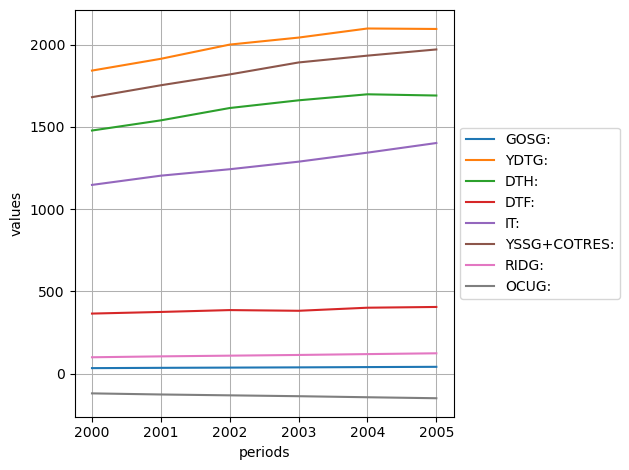
[74]:
<Axes: xlabel='periods', ylabel='values'>
Working with workspaces
As we seen above, IODE operates on objects of 7 different types:
comments
equations
identities
lists
scalars
tables
variables
These are grouped into 7 dictionaries called workspaces.
Load workspaces
To load IODE objects from a binary file (i.e. with extension .cmt, .eqs, .idt, .lst, .scl, .tbl, .var) or from an ASCII file (i.e. with extension .ac, .ae, .ai, .al, .as, .at, .av), use the load() method of the corresponding object. For example:
[75]:
# ---- load equations, identities, scalars and variables ----
from iode import comments, equations, identities, lists, scalars, tables, variables

# Note: test binary and ASCII 'fun' files are located in the 'SAMPLE_DATA_DIR'
#       directory of the 'iode' package
comments.load(f"{SAMPLE_DATA_DIR}/fun.cmt")
equations.load(f"{SAMPLE_DATA_DIR}/fun.eqs")
identities.load(f"{SAMPLE_DATA_DIR}/fun.idt")
lists.load(f"{SAMPLE_DATA_DIR}/fun.lst")
scalars.load(f"{SAMPLE_DATA_DIR}/fun.scl")
tables.load(f"{SAMPLE_DATA_DIR}/fun.tbl")
variables.load(f"{SAMPLE_DATA_DIR}/fun.var")

# ---- print the number of objects present in the above workspaces ----
len(comments), len(equations), len(identities), len(lists), len(scalars), len(tables), len(variables)
Loading C:\soft\miniconda3\Lib\site-packages\iode\tests\data/fun.cmt
317 objects loaded
Loading C:\soft\miniconda3\Lib\site-packages\iode\tests\data/fun.eqs
274 objects loaded
Loading C:\soft\miniconda3\Lib\site-packages\iode\tests\data/fun.idt
48 objects loaded
Loading C:\soft\miniconda3\Lib\site-packages\iode\tests\data/fun.lst
17 objects loaded
Loading C:\soft\miniconda3\Lib\site-packages\iode\tests\data/fun.scl
161 objects loaded
Loading C:\soft\miniconda3\Lib\site-packages\iode\tests\data/fun.tbl
46 objects loaded
Loading C:\soft\miniconda3\Lib\site-packages\iode\tests\data/fun.var
394 objects loaded
[75]:
(317, 274, 48, 17, 161, 46, 394)
Explore workspaces
To get the list of objects names present in a workspace, use the names attribute of the workspace. For example:
[76]:
# get the list of all IODE lists
lists.names
[76]:
['COPY',
 'COPY0',
 'COPY1',
 'ENDO',
 'ENDO0',
 'ENDO1',
 'ENVI',
 'IDT',
 'MAINEQ',
 'MYLIST',
 'TOTAL',
 'TOTAL0',
 'TOTAL1',
 'XENVI',
 'XSCENARIO',
 '_SCAL',
 '_SEARCH']
To check if a name is present in a workspace, use the in operator. For example:
[77]:
if 'ENVI' in lists:
    print("The 'ENVI' IODE list exists")
else:
    print("'ENVI' IODE list not found")
The 'ENVI' IODE list exists
To iterate over names of a workspace, simply use the Python syntax for the for loop:
[78]:
print("Iterate over all IODE lists names in the Lists workspace:")
for name in lists:
    print(name)
Iterate over all IODE lists names in the Lists workspace:
COPY
COPY0
COPY1
ENDO
ENDO0
ENDO1
ENVI
IDT
MAINEQ
MYLIST
TOTAL
TOTAL0
TOTAL1
XENVI
XSCENARIO
_SCAL
_SEARCH
To get the current used sample for the Variables, use the sample attribute of the variables workspace:
[79]:
# current used sample
variables.sample
[79]:
Sample("1960Y1:2015Y1")
Save workspaces
To save the content of a workspace (or a subset of a workspace), use the save() method:
[80]:
# ---- save workspace (or subset) ----
# save the whole workspace
equations.save('equations.eqs')

# save only a subset of the global variables workspace
vars_subset = variables[["ACAF", "ACAG", "AQC", "BQY", "BVY"]]
vars_subset.save('variables_subset.av')

print("Check content of the variables_subset.av file:\n")
with open("variables_subset.av", "r") as f:
    print(f.read())
print()
Saving equations.eqs
274 objects saved
Saving variables_subset.av
Check content of the variables_subset.av file:

sample 1960Y1 2015Y1
ACAF na na na na na na na na na na 1.2130001 5.2020001 9.184 8.0790005 11.332 13.518001 15.784 16.544001 21.489 20.281 21.277 32.417999 24.446999 27.025002 24.504 27.560999 25.542 27.499001 25.353001 17.165001 23.771 26.240999 30.159 34.661999 8.1610022 -13.130997 32.171001 39.935799 29.645657 13.530404919696 10.0466107922005 2.86792273645546 -0.929212509051645 -6.09156498756888 -14.5820944628981 -26.5387895697886 -28.9872879825975 -33.3784257842954 -38.4095177823974 -37.4635096412738 -37.8274288322944 -44.5447926335432 -55.5592898172187 -68.8946543226201 -83.3406251108009 -96.4104198284833
ACAG na na na na na na na na na na -11.028999 -15.847 -19.288002 -21.814999 -25.447002 -24.618999 -27.770998 -28.839001 -29.434998 -30.411001 -30.353001 -41.060997 -31.178001 -32.604 -30.237003 -38.061001 -31.939999 -35.59 -37.238003 -25.991001 -28.1721855713507 -30.934 -40.285999 -43.157997 -16.029003 -41.845993 -40.237 -32.93 -38.345695 -39.8581741316036 -41.534786567348 18.9398011359783 19.9808148751188 21.0205021787734 22.0664755229642 23.1079621640615 24.1296371451098 25.1609090496654 26.1921114843413 27.2299551185986 28.2539289782105 29.2846003640349 30.3239611503116 31.3701388106954 32.4202988291984 33.469601344881
AQC 0.21753037 0.21544869 0.22228125 0.22953896 0.23653506 0.24732406 0.26255098 0.26907021 0.27206925 0.27986595 0.29396999 0.31906503 0.3426649 0.36655167 0.42489415 0.49478459 0.53812659 0.5841772 0.61441606 0.64528418 0.68947881 0.73596764 0.77532566 0.82384807 0.85829282 0.90006256 0.92794591 0.93221092 0.92874223 0.9445076 1 1.0628064 1.1102825 1.1532652 1.1571276 1.1616869 1.1580297 1.201328 1.2031082 1.34296996567459 1.33860285536454 1.37918824681718 1.40881646814855 1.4197045826264 1.40065205989326 1.39697298498842 1.39806354127729 1.40791333507892 1.42564487943834 1.44633167140609 1.46286836974508 1.4822736109441 1.51366597504599 1.55803878946449 1.61318116991651 1.67429057570213
BQY 31.777023 30.852692 30.352686 27.369537 26.937241 35.434574 37.147881 39.505711 42.182659 43.180264 53.083984 49.670918 53.546627 49.331879 50.91983 49.630653 53.96249 40.783443 35.963261 12.621698 -9.930582 -11.615362 -44.158623 -48.221375 -43.152462 -57.944221 -35.790237 -21.710344 -20.180235 -11.333452 -34.099998 -1.2597286 -13.746386 52.161541 66.625153 91.089355 104.67634 113.51928 116.18705 117.908447093342 119.955089852255 121.37741690021 121.700965506023 122.433025255743 124.490157052046 127.572355095553 129.818419511458 131.31355487699 132.020462612763 132.709142263746 133.959190039522 135.075585222668 135.597702367503 135.753159667506 135.968846903397 136.672483513679
BVY 7.1999998 7.0999999 7.1000004 6.6000004 6.8000002 9.3999996 10.3 11.3 12.4 13.3 17.200001 17 19.5 19.200001 22.300001 24.4 28.5 23.099998 21.299999 7.7999992 -6.3999977 -7.9000015 -32.100002 -37.099998 -34.900002 -49.699997 -31.799999 -19.700005 -18.699997 -10.987999 -34.099997 -1.3000031 -14.699997 58.100002 75.900002 105.5 123.2 135.6192 140.73978 144.858781845561 150.053352305841 155.895061264049 160.228327009897 164.690028964993 169.072563292021 173.128489782561 176.73460923165 180.338756120558 184.785317603043 189.533437819158 194.344845745399 199.148256821389 204.263448922459 210.010481935745 216.588822212895 224.043770177584
Workspace subsets
IODE workspaces can contains a lot objects and it can be sometimes easier to work on a subset of the objects present in a workspace. To get a subset of an IODE workspace, a pattern can be passed to the [] operator. A (sub-)pattern is a list of characters representing a group of object names. It includes some special characters which have a special meaning:
*: any character sequence, even empty?: any character (one and only one)@: any alphanumerical char [A-Za-z0-9]&: any non alphanumerical char|: any alphanumeric character or none at the beginning and end of a string!: any non-alphanumeric character or none at the beginning and end of a string\: escape the next character
The pattern can contain sub-patterns, as well as, object names. The sub-patterns and object names are separated by a separator character which is either:
a whitespace
' 'a comma
,a semi-colon
;a tabulation
\ta newline
\n
Note that the pattern can contain references to IODE lists which are prefixed with the symbol $:
[81]:
vars_subset = variables["A*;*_"]
vars_subset
[81]:
Workspace: Variables
nb variables: 33
filename: c:\soft\miniconda3\Lib\site-packages\iode\tests\data\fun.var
description: Modèle fun - Simulation 1
sample: 1960Y1:2015Y1
mode: LEVEL

 name   1960Y1  1961Y1  1962Y1  1963Y1  1964Y1  ...      2010Y1          2011Y1          2012Y1          2013Y1          2014Y1          2015Y1
ACAF        na      na      na      na      na  ...       -37.83          -44.54          -55.56          -68.89          -83.34          -96.41
ACAG        na      na      na      na      na  ...        28.25           29.28           30.32           31.37           32.42           33.47
AOUC        na    0.25    0.25    0.26    0.28  ...         1.31            1.33            1.36            1.39            1.42            1.46
AOUC_       na      na      na      na      na  ...         1.25            1.27            1.30            1.34            1.37            1.41
AQC       0.22    0.22    0.22    0.23    0.24  ...         1.46            1.48            1.51            1.56            1.61            1.67
...        ...     ...     ...     ...     ...  ...          ...             ...             ...             ...             ...             ...
WCF_    193.41  205.78  226.79  250.05  286.84  ...      5170.60         5340.61         5577.10         5872.12         6199.43         6531.10
WIND_    69.98   72.09   75.96   78.14   82.12  ...      1301.03         1338.25         1389.28         1455.12         1532.45         1615.10
WNF_    156.39  164.81  181.95  198.53  224.50  ...      3249.75         3356.81         3505.67         3691.39         3897.45         4106.27
YDH_    439.50  462.93  493.99  530.13  587.08  ...     10995.83        11398.84        11895.99        12481.62        13127.32        13792.13
ZZF_      0.69    0.69    0.69    0.69    0.69  ...         0.69            0.69            0.69            0.69            0.69            0.69
[82]:
lists["ENVI"]
[82]:
['EX',
 'PWMAB',
 'PWMS',
 'PWXAB',
 'PWXS',
 'QWXAB',
 'QWXS',
 'POIL',
 'NATY',
 'TFPFHP_']
[83]:
vars_subset = variables["A*;$ENVI"]
vars_subset
[83]:
Workspace: Variables
nb variables: 15
filename: c:\soft\miniconda3\Lib\site-packages\iode\tests\data\fun.var
description: Modèle fun - Simulation 1
sample: 1960Y1:2015Y1
mode: LEVEL

  name  1960Y1  1961Y1  1962Y1  1963Y1  1964Y1  ...     2010Y1  2011Y1  2012Y1  2013Y1  2014Y1  2015Y1
ACAF        na      na      na      na      na  ...     -37.83  -44.54  -55.56  -68.89  -83.34  -96.41
ACAG        na      na      na      na      na  ...      28.25   29.28   30.32   31.37   32.42   33.47
AOUC        na    0.25    0.25    0.26    0.28  ...       1.31    1.33    1.36    1.39    1.42    1.46
AOUC_       na      na      na      na      na  ...       1.25    1.27    1.30    1.34    1.37    1.41
AQC       0.22    0.22    0.22    0.23    0.24  ...       1.46    1.48    1.51    1.56    1.61    1.67
...        ...     ...     ...     ...     ...  ...        ...     ...     ...     ...     ...     ...
PWXAB     0.23    0.23    0.23    0.23    0.23  ...       1.44    1.46    1.49    1.51    1.54    1.57
PWXS      0.21    0.21    0.21    0.21    0.21  ...       1.70    1.73    1.76    1.79    1.82    1.85
QWXAB     0.44    0.44    0.44    0.44    0.44  ...       4.38    4.63    4.88    5.15    5.43    5.73
QWXS      0.55    0.55    0.55    0.55    0.55  ...       1.77    1.83    1.88    1.94    2.00    2.06
TFPFHP_   0.39    0.40    0.42    0.43    0.44  ...       1.10    1.11    1.12    1.13    1.14    1.15
Get - add - update - delete objects in a workspaces
In a similar way to Python dictionaries, you can get, add, update and delete IODE objects in a workspace using the [] operator.
To extract an IODE object from a workspace, use the syntax:
my_obj = workspace[name].To add an IODE object to a workspace, use the syntax:
workspace[new_name] = new_obj.To update an IODE object in a workspace, use the syntax:
workspace[name] = new_value.To delete an IODE object from a workspace, use the syntax:
del workspace[name].
To add or update IODE objects using:
a pandas Series or DataFrame, see the pandas tutorial.
an larray Array, see the larray tutorial.
a numpy ndarray, see the numpy tutorial.
Comments
Add one comment:
[84]:
comments["NEW"] = "A new comment"
comments["NEW"]
[84]:
'A new comment'
Update a comment:
[85]:
comments["NEW"] = "New Value"
comments["NEW"]
[85]:
'New Value'
Update multiple comments at once:
[86]:
# 1) using a dict of values
values = {"AOUC": "Updated AOUC from dict", "ACAF": "Updated ACAF from dict",
          "ACAG": "Updated ACAG from dict"}
comments["ACAF, ACAG, AOUC"] = values
comments["ACAF, ACAG, AOUC"]
[86]:
Workspace: Comments
nb comments: 3
filename: c:\soft\miniconda3\Lib\site-packages\iode\tests\data\fun.cmt

name           comments
ACAF    Updated ACAF from dict
ACAG    Updated ACAG from dict
AOUC    Updated AOUC from dict
[87]:
# 2) using another Comments database (subset)
comments_subset = comments["ACAF, ACAG, AOUC"].copy()
comments_subset["ACAF"] = "Updated ACAF from another iode Comments database"
comments_subset["ACAG"] = "Updated ACAG from another iode Comments database"
comments_subset["AOUC"] = "Updated AOUC from another iode Comments database"
comments["ACAF, ACAG, AOUC"] = comments_subset
comments["ACAF, ACAG, AOUC"]
[87]:
Workspace: Comments
nb comments: 3
filename: c:\soft\miniconda3\Lib\site-packages\iode\tests\data\fun.cmt

name                        comments
ACAF    Updated ACAF from another iode Comments database
ACAG    Updated ACAG from another iode Comments database
AOUC    Updated AOUC from another iode Comments database
Delete a comment:
[88]:
comments.get_names("A*")
[88]:
['ACAF', 'ACAG', 'AOUC', 'AQC']
[89]:
del comments["ACAF"]
comments.get_names("A*")
[89]:
['ACAG', 'AOUC', 'AQC']
Equations
Add one equation:
[90]:
equations["TEST"] = "TEST := 0"
equations["TEST"]
[90]:
Equation(endogenous = 'TEST',
         lec = 'TEST := 0',
         method = 'LSQ',
         from_period = '1960Y1',
         to_period = '2015Y1')
Update an equation:
[91]:
equations["ACAF"]
[91]:
Equation(endogenous = 'ACAF',
         lec = '(ACAF/VAF[-1]) :=acaf1+acaf2*GOSF[-1]+\nacaf4*(TIME=1995)',
         method = 'LSQ',
         from_period = '1980Y1',
         to_period = '1996Y1',
         block = 'ACAF',
         tests = {corr = 1,
                  dw = 2.32935,
                  fstat = 32.2732,
                  loglik = 83.8075,
                  meany = 0.00818467,
                  r2 = 0.821761,
                  r2adj = 0.796299,
                  ssres = 5.19945e-05,
                  stderr = 0.00192715,
                  stderrp = 23.5458,
                  stdev = 0.0042699},
         date = '12-06-1998')
[92]:
# update only the LEC
equations["ACAF"] = "(ACAF/VAF[-1]) := acaf1 + acaf2 * GOSF[-1] + acaf4 * (TIME=1995)"
equations["ACAF"]
[92]:
Equation(endogenous = 'ACAF',
         lec = '(ACAF/VAF[-1]) := acaf1 + acaf2 * GOSF[-1] + acaf4 * (TIME=1995)',
         method = 'LSQ',
         from_period = '1980Y1',
         to_period = '1996Y1',
         block = 'ACAF',
         tests = {corr = 1,
                  dw = 2.32935,
                  fstat = 32.2732,
                  loglik = 83.8075,
                  meany = 0.00818467,
                  r2 = 0.821761,
                  r2adj = 0.796299,
                  ssres = 5.19945e-05,
                  stderr = 0.00192715,
                  stderrp = 23.5458,
                  stdev = 0.0042699},
         date = '12-06-1998')
[93]:
# update block and sample of a block of equations to estimation (dictionary)
estim_sample = "2000Y1:2010Y1"
block = "ACAF; ACAG; AOUC"
for eq_name in block.split(';'):
    equations[eq_name] = {"sample": estim_sample, "block": block}

(equations["ACAF"].sample, equations["ACAG"].sample, equations["AOUC"].sample)
[93]:
(Sample("2000Y1:2010Y1"), Sample("2000Y1:2010Y1"), Sample("2000Y1:2010Y1"))
[94]:
(equations["ACAF"].block, equations["ACAG"].block, equations["AOUC"].block)
[94]:
('ACAF; ACAG; AOUC', 'ACAF; ACAG; AOUC', 'ACAF; ACAG; AOUC')
[95]:
# update lec, method, sample and block
eq = equations["ACAF"]
eq.lec = "(ACAF/VAF[-1]) := acaf2 * GOSF[-1] + acaf4 * (TIME=1995)"
eq.method = EqMethod.MAX_LIKELIHOOD
eq.sample = "1990Y1:2015Y1"
eq.block = "ACAF"
equations["ACAF"]
[95]:
Equation(endogenous = 'ACAF',
         lec = '(ACAF/VAF[-1]) := acaf2 * GOSF[-1] + acaf4 * (TIME=1995)',
         method = 'MAX_LIKELIHOOD',
         from_period = '1990Y1',
         to_period = '2015Y1',
         block = 'ACAF',
         tests = {corr = 1,
                  dw = 2.32935,
                  fstat = 32.2732,
                  loglik = 83.8075,
                  meany = 0.00818467,
                  r2 = 0.821761,
                  r2adj = 0.796299,
                  ssres = 5.19945e-05,
                  stderr = 0.00192715,
                  stderrp = 23.5458,
                  stdev = 0.0042699},
         date = '12-06-1998')
Update multiple equations at once:
[96]:
# 1) using a dict of values
eq_ACAF = Equation("ACAF", "(ACAF/VAF[-1]) :=acaf1+acaf2*GOSF[-1]+ acaf4*(TIME=1995)",
                   method=EqMethod.ZELLNER, from_period='1980Y1', to_period='1996Y1')
eq_ACAG = Equation("ACAG", "ACAG := ACAG[-1]+r VBBP[-1]+(0.006*VBBP[-1]*(TIME=2001)-0.008*(TIME=2008))",
                   method=EqMethod.ZELLNER, from_period='1980Y1', to_period='1996Y1')
eq_AOUC = Equation("AOUC", "AOUC:=((WCRH/QL)/(WCRH/QL)[1990Y1])*(VAFF/(VM+VAFF))[-1]+PM*(VM/(VAFF+VM))[-1]",
                   method=EqMethod.ZELLNER, from_period='1980Y1', to_period='1996Y1')
values = {"ACAF": eq_ACAF, "ACAG": eq_ACAG, "AOUC": eq_AOUC}
equations["ACAF, ACAG, AOUC"] = values
equations["ACAF, ACAG, AOUC"]
[96]:
Workspace: Equations
nb equations: 3
filename: c:\usr\Projects\iode-1\doc\source\tutorial\equations.eqs

name                                         lec                                         method     sample      block   fstat   r2adj     dw    loglik  date
ACAF    (ACAF/VAF[-1]) :=acaf1+acaf2*GOSF[-1]+ acaf4*(TIME=1995)                        ZELLNER 1980Y1:1996Y1           0.0000  0.0000  0.0000  0.0000
ACAG    ACAG := ACAG[-1]+r VBBP[-1]+(0.006*VBBP[-1]*(TIME=2001)-0.008*(TIME=2008))      ZELLNER 1980Y1:1996Y1           0.0000  0.0000  0.0000  0.0000
AOUC    AOUC:=((WCRH/QL)/(WCRH/QL)[1990Y1])*(VAFF/(VM+VAFF))[-1]+PM*(VM/(VAFF+VM))[-1]  ZELLNER 1980Y1:1996Y1           0.0000  0.0000  0.0000  0.0000
[97]:
# 2) using another Equations database (subset)
equations_subset = equations["ACAF, ACAG, AOUC"].copy()
for eq_name in equations_subset.names:
    equations_subset[eq_name].method = EqMethod.MAX_LIKELIHOOD
equations["ACAF, ACAG, AOUC"] = equations_subset
equations["ACAF, ACAG, AOUC"]
[97]:
Workspace: Equations
nb equations: 3
filename: c:\usr\Projects\iode-1\doc\source\tutorial\equations.eqs

name                                         lec                                            method          sample      block   fstat   r2adj     dw    loglik  date
ACAF    (ACAF/VAF[-1]) :=acaf1+acaf2*GOSF[-1]+ acaf4*(TIME=1995)                        MAX_LIKELIHOOD  1980Y1:1996Y1           0.0000  0.0000  0.0000  0.0000
ACAG    ACAG := ACAG[-1]+r VBBP[-1]+(0.006*VBBP[-1]*(TIME=2001)-0.008*(TIME=2008))      MAX_LIKELIHOOD  1980Y1:1996Y1           0.0000  0.0000  0.0000  0.0000
AOUC    AOUC:=((WCRH/QL)/(WCRH/QL)[1990Y1])*(VAFF/(VM+VAFF))[-1]+PM*(VM/(VAFF+VM))[-1]  MAX_LIKELIHOOD  1980Y1:1996Y1           0.0000  0.0000  0.0000  0.0000
Delete an equation:
[98]:
equations.get_names("A*")
[98]:
['ACAF', 'ACAG', 'AOUC']
[99]:
del equations["ACAF"]
equations.get_names("A*")
[99]:
['ACAG', 'AOUC']
[100]:
# store an equation in a Python variable
eq = equations["DEBT"]
eq
c:\soft\Miniconda3\Lib\site-packages\iode\objects\equation.py:1277: UserWarning: 'sample' is not defined
  return self._cy_equation._repr_()
[100]:
Equation(endogenous = 'DEBT',
         lec = 'd DEBT := OCP-FLG',
         method = 'LSQ',
         comment = ' ',
         block = 'DEBT')
[101]:
# then delete it from the database
del equations["DEBT"]
"DEBT" in equations
[101]:
False
[102]:
# NOTE: the Python variable 'eq' still contains the equation object
eq
[102]:
Equation(endogenous = 'DEBT',
         lec = 'd DEBT := OCP-FLG',
         method = 'LSQ',
         comment = ' ',
         block = 'DEBT')
Identities
Add one identity:
[103]:
identities["BDY"] = "YN - YK"
identities["BDY"]
[103]:
Identity('YN - YK')
Update an identity:
[104]:
identities["AOUC"]
[104]:
Identity('((WCRH/QL)/(WCRH/QL)[1990Y1])*(VAFF/(VM+VAFF))[-1]+PM*(VM/(VM+VAFF))[-1]')
[105]:
identities["AOUC"] = '(WCRH / WCRH[1990Y1]) * (VAFF / (VM+VAFF))[-1] + PM * (VM / (VM+VAFF))[-1]'
identities["AOUC"]
[105]:
Identity('(WCRH / WCRH[1990Y1]) * (VAFF / (VM+VAFF))[-1] + PM * (VM / (VM+VAFF))[-1]')
[106]:
# or equivalently
idt = identities["AOUC"]
idt.lec = "(WCRH / WCRH[1990Y1]) * (VAFF / (VM+VAFF))[-1]"
identities["AOUC"]
[106]:
Identity('(WCRH / WCRH[1990Y1]) * (VAFF / (VM+VAFF))[-1]')
Update multiple identities at once:
[107]:
# 1) using a dict of values
values = {"GAP2": "0.9 * 100*(QAFF_/(Q_F+Q_I))", "GAP_": "0.9 * 100*((QAF_/Q_F)-1)",
          "GOSFR": "0.9 * (GOSF/VAF_)"}
identities["GAP2, GAP_, GOSFR"] = values
identities["GAP2, GAP_, GOSFR"]
[107]:
Workspace: Identities
nb identities: 3
filename: c:\soft\miniconda3\Lib\site-packages\iode\tests\data\fun.idt

 name            identities
GAP2    0.9 * 100*(QAFF_/(Q_F+Q_I))
GAP_    0.9 * 100*((QAF_/Q_F)-1)
GOSFR   0.9 * (GOSF/VAF_)
[108]:
# 2) using another Identities database (subset)
identities_subset = identities["GAP2, GAP_, GOSFR"].copy()
identities_subset["GAP2"] = "0.7 * 100*(QAFF_/(Q_F+Q_I))"
identities_subset["GAP_"] = "0.7 * 100*((QAF_/Q_F)-1)"
identities_subset["GOSFR"] = "0.7 * (GOSF/VAF_)"
identities["GAP2, GAP_, GOSFR"] = identities_subset
identities["GAP2, GAP_, GOSFR"]
[108]:
Workspace: Identities
nb identities: 3
filename: c:\soft\miniconda3\Lib\site-packages\iode\tests\data\fun.idt

 name            identities
GAP2    0.7 * 100*(QAFF_/(Q_F+Q_I))
GAP_    0.7 * 100*((QAF_/Q_F)-1)
GOSFR   0.7 * (GOSF/VAF_)
Delete an identity:
[109]:
identities.get_names("W*")
[109]:
['W', 'WBGR', 'WCRH', 'WMINR', 'WO']
[110]:
del identities["W"]
identities.get_names("W*")
[110]:
['WBGR', 'WCRH', 'WMINR', 'WO']
[111]:
# create a new identity and store it in a Python variable
idt = Identity("YN - YK")
idt
[111]:
Identity('YN - YK')
[112]:
# add it to the database
identities["NEW_IDT"] = idt
identities["NEW_IDT"]
[112]:
Identity('YN - YK')
[113]:
# then delete it from the database
del identities["NEW_IDT"]
"NEW_IDT" in identities
[113]:
False
[114]:
# NOTE: the Python variable 'idt' still contains the identity object
idt
[114]:
Identity('YN - YK')
Lists
Add one list:
[115]:
# --- by passing a string
lists["A_VAR"] = "ACAF;ACAG;AOUC;AOUC_;AQC"
lists["A_VAR"]
[115]:
['ACAF', 'ACAG', 'AOUC', 'AOUC_', 'AQC']
[116]:
# --- by passing a Python list
b_vars = variables.get_names("B*")
b_vars
[116]:
['BENEF', 'BQY', 'BRUGP', 'BVY']
[117]:
lists["B_VAR"] = b_vars
lists["B_VAR"]
[117]:
['BENEF', 'BQY', 'BRUGP', 'BVY']
Update a list:
[118]:
# --- by passing a string
lists["A_VAR"] = "ACAF;ACAG;AOUC;AQC"
lists["A_VAR"]
[118]:
['ACAF', 'ACAG', 'AOUC', 'AQC']
[119]:
# --- by passing a Python list
b_y_vars = variables.get_names("B*Y")
b_y_vars
[119]:
['BQY', 'BVY']
[120]:
lists["B_VAR"] = b_y_vars
lists["B_VAR"]
[120]:
['BQY', 'BVY']
Update multiple lists at once:
[121]:
# 1) using a dict of values
values = {"ENVI": "PWMAB; PWMS; PWXAB; PWXS; QWXAB; QWXS; POIL; NATY",
          "IDT": "FLGR; KL; PROD; QL; RDEBT; RENT; RLBER; SBGX; WCRH; IUGR; SBGXR; WBGR; YSFICR",
          "MAINEQ": "NFYH; KNFF; PC; PXAB; PMAB; QXAB; QMAB"}
lists["ENVI, IDT, MAINEQ"] = values
lists["ENVI, IDT, MAINEQ"]
[121]:
Workspace: Lists
nb lists: 3
filename: c:\soft\miniconda3\Lib\site-packages\iode\tests\data\fun.lst
description: Modèle fun

 name                                       lists
ENVI    PWMAB; PWMS; PWXAB; PWXS; QWXAB; QWXS; POIL; NATY
IDT     FLGR; KL; PROD; QL; RDEBT; RENT; RLBER; SBGX; WCRH; IUGR; SBGXR; WBGR; YSFICR
MAINEQ  NFYH; KNFF; PC; PXAB; PMAB; QXAB; QMAB
[122]:
# 2) using another Lists database (subset)
lists_subset = lists["ENVI, IDT, MAINEQ"].copy()
lists_subset["ENVI"] = "PWXAB; PWXS; QWXAB; QWXS"
lists_subset["IDT"] = "PROD; QL; RDEBT; RENT; RLBER; SBGX; WCRH; IUGR; SBGXR"
lists_subset["MAINEQ"] = "PC; PXAB; PMAB"
lists["ENVI, IDT, MAINEQ"] = lists_subset
lists["ENVI, IDT, MAINEQ"]
[122]:
Workspace: Lists
nb lists: 3
filename: c:\soft\miniconda3\Lib\site-packages\iode\tests\data\fun.lst
description: Modèle fun

 name                           lists
ENVI    PWXAB; PWXS; QWXAB; QWXS
IDT     PROD; QL; RDEBT; RENT; RLBER; SBGX; WCRH; IUGR; SBGXR
MAINEQ  PC; PXAB; PMAB
Delete a list:
[123]:
lists.get_names("C*")
[123]:
['COPY', 'COPY0', 'COPY1']
[124]:
del lists["COPY"]
lists.get_names("C*")
[124]:
['COPY0', 'COPY1']
Scalars
Add one scalar:
[125]:
# 1. default relax to 1.0
scalars["a0"] = 0.1
scalars["a0"]
[125]:
Scalar(0.1, 1, na)
[126]:
# 2. value + relax
scalars["a1"] = 0.1, 0.9
scalars["a1"]
[126]:
Scalar(0.1, 0.9, na)
Update a scalar:
[127]:
scalars["acaf1"]
[127]:
Scalar(0.0157684, 1, 0.00136871)
[128]:
# only update the value
scalars["acaf1"] = 0.8
scalars["acaf1"]
[128]:
Scalar(0.8, 1, na)
[129]:
# update value and relax (tuple)
scalars["acaf2"] = 0.8, 0.9
scalars["acaf2"]
[129]:
Scalar(0.8, 0.9, na)
[130]:
# update value and relax (list)
scalars["acaf2"] = (0.7, 0.8)
scalars["acaf2"]
[130]:
Scalar(0.7, 0.8, na)
[131]:
# update value and relax (dictionary)
scalars["acaf3"] = {"relax": 0.9, "value": 0.8}
scalars["acaf3"]
[131]:
Scalar(0.8, 0.9, na)
[132]:
# update value and/or relax (Scalar object)
# NOTE: the standard deviation (std) cannot be changed manually
scalars["acaf4"]
[132]:
Scalar(-0.00850518, 1, 0.0020833)
[133]:
scl = scalars["acaf4"]
scl.value = 0.8
scl.relax = 0.9
scalars["acaf4"]
[133]:
Scalar(0.8, 0.9, na)
Update multiple scalars at once:
[134]:
# 1) using a dict of values
values = {"acaf1": 0.016, "acaf2": (-8.e-04, 0.9), "acaf3": Scalar(2.5)}
scalars["acaf1, acaf2, acaf3"] = values
scalars["acaf1, acaf2, acaf3"]
[134]:
Workspace: Scalars
nb scalars: 3
filename: c:\soft\miniconda3\Lib\site-packages\iode\tests\data\fun.scl

 name    value  relax   std
acaf1    0.0160 1.0000   na
acaf2   -0.0008 0.9000   na
acaf3    2.5000 1.0000   na
[135]:
# 2) using another Scalars database (subset)
scalars_subset = scalars["acaf1, acaf2, acaf3"].copy()
scalars_subset["acaf1"] = 0.02
scalars_subset["acaf2"] = (-5.e-04, 0.94)
scalars_subset["acaf3"] = Scalar(2.9)
scalars["acaf1, acaf2, acaf3"] = scalars_subset
scalars["acaf1, acaf2, acaf3"]
[135]:
Workspace: Scalars
nb scalars: 3
filename: c:\soft\miniconda3\Lib\site-packages\iode\tests\data\fun.scl

 name    value  relax   std
acaf1    0.0200 1.0000   na
acaf2   -0.0005 0.9400   na
acaf3    2.9000 1.0000   na
Delete a scalar:
[136]:
scalars.get_names("a*")
[136]:
['a0', 'a1', 'acaf1', 'acaf2', 'acaf3', 'acaf4']
[137]:
del scalars["acaf4"]
scalars.get_names("a*")
[137]:
['a0', 'a1', 'acaf1', 'acaf2', 'acaf3']
[138]:
# store a scalar in a Python variable
scl = scalars["zkf1"]
scl
[138]:
Scalar(0.201117, 1, 0.375671)
[139]:
# then delete it from the database
del scalars["zkf1"]
"zkf1" in scalars
[139]:
False
[140]:
# NOTE: the Python variable 'scl' still contains the scalar object
scl
[140]:
Scalar(0.201117, 1, 0.375671)
Tables
Create an add a new table:
[141]:
# 1. specify list of line titles and list of LEC expressions
lines_titles = ["GOSG:", "YDTG:", "DTH:", "DTF:", "IT:", "YSSG+COTRES:", "RIDG:", "OCUG:"]
lines_lecs = ["GOSG", "YDTG", "DTH", "DTF", "IT", "YSSG+COTRES", "RIDG", "OCUG"]
tables["TABLE_CELL_LECS"] = {"nb_columns": 2, "table_title": "New Table", "lecs_or_vars": lines_lecs,
                             "lines_titles": lines_titles, "mode": True, "files": True, "date": True}
tables["TABLE_CELL_LECS"]
[141]:
DIVIS | 1              |
TITLE |         "New Table"
----- | ----------------------------
CELL  |                |     "#S"
----- | ----------------------------
CELL  | "GOSG:"        |        GOSG
CELL  | "YDTG:"        |        YDTG
CELL  | "DTH:"         |         DTH
CELL  | "DTF:"         |         DTF
CELL  | "IT:"          |          IT
CELL  | "YSSG+COTRES:" | YSSG+COTRES
CELL  | "RIDG:"        |        RIDG
CELL  | "OCUG:"        |        OCUG
----- | ----------------------------
MODE  |
FILES |
DATE  |

nb lines: 16
nb columns: 2
language: 'ENGLISH'
gridx: 'MAJOR'
gridy: 'MAJOR'
graph_axis: 'VALUES'
graph_alignment: 'LEFT'
[142]:
# 2. specify list of variables
vars_list = ["GOSG", "YDTG", "DTH", "DTF", "IT", "YSSG", "COTRES", "RIDG", "OCUG", "$ENVI"]
tables["TABLE_VARS"] = {"nb_columns": 2, "table_title": "New Table", "lecs_or_vars": vars_list,
                        "mode": True, "files": True, "date": True}
tables["TABLE_VARS"]
[142]:
DIVIS | 1                                                                    |
TITLE |                                  "New Table"
----- | -----------------------------------------------------------------------------
CELL  |                                                                      |  "#S"
----- | -----------------------------------------------------------------------------
CELL  | "Bruto exploitatie-overschot: overheid (= afschrijvingen)."          |   GOSG
CELL  | "Overheid: geïnde indirecte belastingen."                            |   YDTG
CELL  | "Totale overheid: directe belasting van de gezinnen."                |    DTH
CELL  | "Totale overheid: directe vennootschapsbelasting."                   |    DTF
CELL  | "Totale indirecte belastingen."                                      |     IT
CELL  | "Globale overheid: ontvangen sociale zekerheidsbijdragen."           |   YSSG
CELL  | "Cotisation de responsabilisation."                                  | COTRES
CELL  | "Overheid: inkomen uit vermogen."                                    |   RIDG
CELL  | "Globale overheid: saldo van de ontvangen lopendeoverdrachten."      |   OCUG
CELL  | "Index wereldprijs - uitvoer van niet-energieprodukten, inUSD."      |  PWXAB
CELL  | "Index wereldprijs - uitvoer van diensten, in USD."                  |   PWXS
CELL  | "Indicator van het volume van de wereldvraag naar goederen,1985=1."  |  QWXAB
CELL  | "Indicator van het volume van de wereldvraag naar diensten,1985=1."  |   QWXS
----- | -----------------------------------------------------------------------------
MODE  |
FILES |
DATE  |

nb lines: 21
nb columns: 2
language: 'ENGLISH'
gridx: 'MAJOR'
gridy: 'MAJOR'
graph_axis: 'VALUES'
graph_alignment: 'LEFT'
Update a table:
[143]:
table = tables["TABLE_CELL_LECS"]
table
[143]:
DIVIS | 1              |
TITLE |         "New Table"
----- | ----------------------------
CELL  |                |     "#S"
----- | ----------------------------
CELL  | "GOSG:"        |        GOSG
CELL  | "YDTG:"        |        YDTG
CELL  | "DTH:"         |         DTH
CELL  | "DTF:"         |         DTF
CELL  | "IT:"          |          IT
CELL  | "YSSG+COTRES:" | YSSG+COTRES
CELL  | "RIDG:"        |        RIDG
CELL  | "OCUG:"        |        OCUG
----- | ----------------------------
MODE  |
FILES |
DATE  |

nb lines: 16
nb columns: 2
language: 'ENGLISH'
gridx: 'MAJOR'
gridy: 'MAJOR'
graph_axis: 'VALUES'
graph_alignment: 'LEFT'
[144]:
table.graph_axis
[144]:
'VALUES'
[145]:
from iode import TableGraphAxis
# set graph axis type
table.graph_axis = TableGraphAxis.SEMILOG
table.graph_axis
[145]:
'SEMILOG'
[146]:
# get the first line
table[0]
[146]:
New Table
[147]:
# get the last line
table[-1]
[147]:
<DATE>
[148]:
# delete last line
del table[-1]
table
[148]:
DIVIS | 1              |
TITLE |         "New Table"
----- | ----------------------------
CELL  |                |     "#S"
----- | ----------------------------
CELL  | "GOSG:"        |        GOSG
CELL  | "YDTG:"        |        YDTG
CELL  | "DTH:"         |         DTH
CELL  | "DTF:"         |         DTF
CELL  | "IT:"          |          IT
CELL  | "YSSG+COTRES:" | YSSG+COTRES
CELL  | "RIDG:"        |        RIDG
CELL  | "OCUG:"        |        OCUG
----- | ----------------------------
MODE  |
FILES |

nb lines: 15
nb columns: 2
language: 'ENGLISH'
gridx: 'MAJOR'
gridy: 'MAJOR'
graph_axis: 'SEMILOG'
graph_alignment: 'LEFT'
[149]:
# get index of line containing YSSG+COTRES
index = table.index("YSSG+COTRES")
index
[149]:
9
[150]:
table[index]
[150]:
('"YSSG+COTRES:"', 'YSSG+COTRES')
[151]:
# get line type
table[index].line_type
[151]:
'CELL'
[152]:
# get line graph type
table[index].graph_type
[152]:
'LINE'
[153]:
# know if axis is left
table[index].axis_left
[153]:
True
[154]:
# update cells
# double quotes "    -> STRING cell
# no double quotes   -> LEC cell
table[index] = ('"YSSG:"', 'YSSG')
table[index]
[154]:
('"YSSG:"', 'YSSG')
[155]:
# insert a new title line surrounded by two separator lines
table.insert(index + 1, '-')
table.insert(index + 2, "New Title")
table.insert(index + 3, '-')
table
[155]:
DIVIS | 1       |
TITLE |  "New Table"
----- | --------------
CELL  |         | "#S"
----- | --------------
CELL  | "GOSG:" | GOSG
CELL  | "YDTG:" | YDTG
CELL  | "DTH:"  |  DTH
CELL  | "DTF:"  |  DTF
CELL  | "IT:"   |   IT
CELL  | "YSSG:" | YSSG
----- | --------------
TITLE |  "New Title"
----- | --------------
CELL  | "RIDG:" | RIDG
CELL  | "OCUG:" | OCUG
----- | --------------
MODE  |
FILES |

nb lines: 18
nb columns: 2
language: 'ENGLISH'
gridx: 'MAJOR'
gridy: 'MAJOR'
graph_axis: 'SEMILOG'
graph_alignment: 'LEFT'
[156]:
# append a new sepatator line
table += '-'
table
[156]:
DIVIS | 1       |
TITLE |  "New Table"
----- | --------------
CELL  |         | "#S"
----- | --------------
CELL  | "GOSG:" | GOSG
CELL  | "YDTG:" | YDTG
CELL  | "DTH:"  |  DTH
CELL  | "DTF:"  |  DTF
CELL  | "IT:"   |   IT
CELL  | "YSSG:" | YSSG
----- | --------------
TITLE |  "New Title"
----- | --------------
CELL  | "RIDG:" | RIDG
CELL  | "OCUG:" | OCUG
----- | --------------
MODE  |
FILES |
----- | --------------

nb lines: 19
nb columns: 2
language: 'ENGLISH'
gridx: 'MAJOR'
gridy: 'MAJOR'
graph_axis: 'SEMILOG'
graph_alignment: 'LEFT'
[157]:
tables["TABLE_CELL_LECS"]
[157]:
DIVIS | 1       |
TITLE |  "New Table"
----- | --------------
CELL  |         | "#S"
----- | --------------
CELL  | "GOSG:" | GOSG
CELL  | "YDTG:" | YDTG
CELL  | "DTH:"  |  DTH
CELL  | "DTF:"  |  DTF
CELL  | "IT:"   |   IT
CELL  | "YSSG:" | YSSG
----- | --------------
TITLE |  "New Title"
----- | --------------
CELL  | "RIDG:" | RIDG
CELL  | "OCUG:" | OCUG
----- | --------------
MODE  |
FILES |
----- | --------------

nb lines: 19
nb columns: 2
language: 'ENGLISH'
gridx: 'MAJOR'
gridy: 'MAJOR'
graph_axis: 'SEMILOG'
graph_alignment: 'LEFT'
Update multiple tables at once:
[158]:
# 1) using a dict of values
table_C8_1 = tables["C8_1"].copy()
table_C8_1.title = table_C8_1.title + " (copy)"
table_C8_2 = tables["C8_2"].copy()
table_C8_2.title = table_C8_2.title + " (copy)"
table_C8_3 = tables["C8_3"].copy()
table_C8_3.title = table_C8_3.title + " (copy)"

values = {"C8_1": table_C8_1, "C8_2": table_C8_2, "C8_3": table_C8_3}
tables["C8_1, C8_2, C8_3"] = values
tables["C8_1, C8_2, C8_3"]
[158]:
Workspace: Tables
nb tables: 3
filename: c:\soft\miniconda3\Lib\site-packages\iode\tests\data\fun.tbl

name                   table titles
C8_1    Déterminants de l'output potentiel (copy)
C8_2    Déterminants de la productivité (copy)
C8_3    Output gap (copy)
[159]:
# 2) using another tables database (subset)
tables_subset = tables["C8_1, C8_2, C8_3"].copy()
for tbl_name in tables_subset.names:
    title = tables_subset[tbl_name].title
    tables_subset[tbl_name].title = title.replace("(copy)", "(detached subset)")
tables["C8_1, C8_2, C8_3"] = tables_subset
tables["C8_1, C8_2, C8_3"]
[159]:
Workspace: Tables
nb tables: 3
filename: c:\soft\miniconda3\Lib\site-packages\iode\tests\data\fun.tbl

name                        table titles
C8_1    Déterminants de l'output potentiel (detached subset)
C8_2    Déterminants de la productivité (detached subset)
C8_3    Output gap (detached subset)
Delete a table:
[160]:
tables.get_names("G*")
[160]:
['GAP', 'GDP', 'GFR', 'GFRLEVEL', 'GFRPC', 'GROWTH']
[161]:
del tables["GFRLEVEL"]
tables.get_names("G*")
[161]:
['GAP', 'GDP', 'GFR', 'GFRPC', 'GROWTH']
[162]:
# store a table in a Python variable
tbl = tables["MULT1FR"]
tbl
[162]:
DIVIS | 1                                              |
TITLE |         "Principaux indicateurs : montants absolus"
----- | -----------------------------------------------------------
CELL  | " "                                            | "#s"
----- | -----------------------------------------------------------
CELL  | "1. Demande globale"                           |
CELL  | "       Consommation privée"                   |         QC
CELL  | "       Consommation publique"                 |         QG
CELL  | "       Formation brute de capital fixe"       |         QI
CELL  | "            - Entreprises"                    |        QIF
CELL  | "            - Etat"                           |        QIG
CELL  | "            - Logements"                      |        QI5
CELL  | "       Exportations de biens et services"     |         QX
CELL  | "       Importations de biens et services"     |         QM
CELL  | "       Produit Intérieur Brut"                |       QBBP
CELL  | "       Produit National Brut"                 |       QBNP
CELL  | "2. Marché du travail"                         |
CELL  | "       Emploi total"                          |    NATY-UY
CELL  | "         Entreprises"                         |    NFY+NIY
CELL  | "         Etat"                                |        NGY
CELL  | "3. Prix, salaires et revenus"                 |
CELL  | "       Salaire coût horaire"                  |       WCRH
CELL  | "       Salaire coût réel horaire"             |    WCRH/PC
CELL  | "       Déflateur de la consommation privée"   |         PC
CELL  | "       Coûts salariaux unitaires (apparents)" |  WCRH/PROD
CELL  | "       Coûts salariaux unitaires (techn.)"    |    WCRH/QL
CELL  | "       Prix des importations"                 |         PM
CELL  | "       Coûts totaux par unité produite "      |       AOUC
CELL  | "       Prix des exportations de biens"        |       PXAB
CELL  | "       Termes de l'échange (PX/PM)"           |      PX/PM
CELL  | "       Revenu disponible réel des ménages"    |     YDH/PC
CELL  | "4. Entreprises"                               |
CELL  | "       Valeur ajoutée (prix constants)"       |       QAF_
CELL  | "       Déflateur de la valeur ajoutée"        |       PAF_
CELL  | "       Valeur ajoutée potentielle"            |        Q_F
CELL  | "       Stock de capital"                      |       KNFY
CELL  | "5. Productivités du travail"                  |
CELL  | "       Productivité horaire apparente"        |       PROD
CELL  | "       Productivité horaire technique"        |         QL
CELL  | "       Productivité par tête "                | QAF_/(NFY)
----- | -----------------------------------------------------------
MODE  |
FILES |
DATE  |

nb lines: 43
nb columns: 2
language: 'ENGLISH'
gridx: 'MAJOR'
gridy: 'MAJOR'
graph_axis: 'VALUES'
graph_alignment: 'LEFT'
[163]:
# then delete it from the database
del tables["MULT1FR"]
"MULT1FR" in tables
[163]:
False
[164]:
# NOTE: the Python variable 'tbl' still contains the table object
tbl
[164]:
DIVIS | 1                                              |
TITLE |         "Principaux indicateurs : montants absolus"
----- | -----------------------------------------------------------
CELL  | " "                                            | "#s"
----- | -----------------------------------------------------------
CELL  | "1. Demande globale"                           |
CELL  | "       Consommation privée"                   |         QC
CELL  | "       Consommation publique"                 |         QG
CELL  | "       Formation brute de capital fixe"       |         QI
CELL  | "            - Entreprises"                    |        QIF
CELL  | "            - Etat"                           |        QIG
CELL  | "            - Logements"                      |        QI5
CELL  | "       Exportations de biens et services"     |         QX
CELL  | "       Importations de biens et services"     |         QM
CELL  | "       Produit Intérieur Brut"                |       QBBP
CELL  | "       Produit National Brut"                 |       QBNP
CELL  | "2. Marché du travail"                         |
CELL  | "       Emploi total"                          |    NATY-UY
CELL  | "         Entreprises"                         |    NFY+NIY
CELL  | "         Etat"                                |        NGY
CELL  | "3. Prix, salaires et revenus"                 |
CELL  | "       Salaire coût horaire"                  |       WCRH
CELL  | "       Salaire coût réel horaire"             |    WCRH/PC
CELL  | "       Déflateur de la consommation privée"   |         PC
CELL  | "       Coûts salariaux unitaires (apparents)" |  WCRH/PROD
CELL  | "       Coûts salariaux unitaires (techn.)"    |    WCRH/QL
CELL  | "       Prix des importations"                 |         PM
CELL  | "       Coûts totaux par unité produite "      |       AOUC
CELL  | "       Prix des exportations de biens"        |       PXAB
CELL  | "       Termes de l'échange (PX/PM)"           |      PX/PM
CELL  | "       Revenu disponible réel des ménages"    |     YDH/PC
CELL  | "4. Entreprises"                               |
CELL  | "       Valeur ajoutée (prix constants)"       |       QAF_
CELL  | "       Déflateur de la valeur ajoutée"        |       PAF_
CELL  | "       Valeur ajoutée potentielle"            |        Q_F
CELL  | "       Stock de capital"                      |       KNFY
CELL  | "5. Productivités du travail"                  |
CELL  | "       Productivité horaire apparente"        |       PROD
CELL  | "       Productivité horaire technique"        |         QL
CELL  | "       Productivité par tête "                | QAF_/(NFY)
----- | -----------------------------------------------------------
MODE  |
FILES |
DATE  |

nb lines: 43
nb columns: 2
language: 'ENGLISH'
gridx: 'MAJOR'
gridy: 'MAJOR'
graph_axis: 'VALUES'
graph_alignment: 'LEFT'
Variables
Get variable:
[165]:
# get the value for a single period -> float
variables["ACAF", "1990Y1"]
[165]:
23.771
[166]:
# get the values for all periods -> Variables
variables["ACAF"]
[166]:
Workspace: Variables
nb variables: 1
filename: c:\soft\miniconda3\Lib\site-packages\iode\tests\data\fun.var
description: Modèle fun - Simulation 1
sample: 1960Y1:2015Y1
mode: LEVEL

name    1960Y1  1961Y1  1962Y1  1963Y1  1964Y1  1965Y1  ...     2009Y1  2010Y1  2011Y1  2012Y1  2013Y1  2014Y1  2015Y1
ACAF        na      na      na      na      na      na  ...     -37.46  -37.83  -44.54  -55.56  -68.89  -83.34  -96.41
[167]:
# get the values for a range of periods -> Variables
variables["ACAF", "1990Y1:2000Y1"]
[167]:
Workspace: Variables
nb variables: 1
filename: c:\soft\miniconda3\Lib\site-packages\iode\tests\data\fun.var
description: Modèle fun - Simulation 1
sample: 1990Y1:2000Y1
mode: LEVEL
name 1990Y1 1991Y1 1992Y1 1993Y1 1994Y1 1995Y1 1996Y1 1997Y1 1998Y1 1999Y1 2000Y1
ACAF 23.77 26.24 30.16 34.66 8.16 -13.13 32.17 39.94 29.65 13.53 10.05
[168]:
# get the values for a list non-contiguous periods -> pandas Series
variables["ACAF", ["1990Y1", "1995Y1", "2000Y1"]]
[168]:
time
1990Y1 23.771000
1995Y1 -13.130997
2000Y1 10.046611
Name: ACAF, dtype: float64
Get values for a single period:
[169]:
variables[:, "1990Y1"]
[169]:
Workspace: Variables
nb variables: 394
filename: c:\soft\miniconda3\Lib\site-packages\iode\tests\data\fun.var
description: Modèle fun - Simulation 1
sample: 1990Y1:1990Y1
mode: LEVEL
name 1990Y1
ACAF 23.77
ACAG -28.17
AOUC 1.00
AOUC_ 0.94
AQC 1.00
... ...
ZJ 1.09
ZKF 0.81
ZKFO 1.00
ZX 0.00
ZZF_ 0.69
or equivalently:
[170]:
variables["*", "1990Y1"]
[170]:
Workspace: Variables
nb variables: 394
filename: c:\soft\miniconda3\Lib\site-packages\iode\tests\data\fun.var
description: Modèle fun - Simulation 1
sample: 1990Y1:1990Y1
mode: LEVEL
name 1990Y1
ACAF 23.77
ACAG -28.17
AOUC 1.00
AOUC_ 0.94
AQC 1.00
... ...
ZJ 1.09
ZKF 0.81
ZKFO 1.00
ZX 0.00
ZZF_ 0.69
Add one variable:
[171]:
# 1) same value for all periods
# NOTE: you can also use NA from iode to set a variable value to NaN
variables["A0"] = np.nan
variables["A0"]
[171]:
Workspace: Variables
nb variables: 1
filename: c:\soft\miniconda3\Lib\site-packages\iode\tests\data\fun.var
description: Modèle fun - Simulation 1
sample: 1960Y1:2015Y1
mode: LEVEL
name 1960Y1 1961Y1 1962Y1 1963Y1 1964Y1 1965Y1 ... 2009Y1 2010Y1 2011Y1 2012Y1 2013Y1 2014Y1 2015Y1
A0 na na na na na na ... na na na na na na na
[172]:
# 2) LEC expression
variables["A1"] = "t + 10"
variables["A1"]
[172]:
Workspace: Variables
nb variables: 1
filename: c:\soft\miniconda3\Lib\site-packages\iode\tests\data\fun.var
description: Modèle fun - Simulation 1
sample: 1960Y1:2015Y1
mode: LEVEL
name 1960Y1 1961Y1 1962Y1 1963Y1 1964Y1 1965Y1 ... 2009Y1 2010Y1 2011Y1 2012Y1 2013Y1 2014Y1 2015Y1
A1 10.00 11.00 12.00 13.00 14.00 15.00 ... 59.00 60.00 61.00 62.00 63.00 64.00 65.00
[173]:
# 3) list of values for each period
values = list(range(variables.nb_periods))
values[0] = NA
values[-1] = np.nan
variables["A2"] = values
variables["A2"]
[173]:
Workspace: Variables
nb variables: 1
filename: c:\soft\miniconda3\Lib\site-packages\iode\tests\data\fun.var
description: Modèle fun - Simulation 1
sample: 1960Y1:2015Y1
mode: LEVEL
name 1960Y1 1961Y1 1962Y1 1963Y1 1964Y1 1965Y1 ... 2009Y1 2010Y1 2011Y1 2012Y1 2013Y1 2014Y1 2015Y1
A2 na 1.00 2.00 3.00 4.00 5.00 ... 49.00 50.00 51.00 52.00 53.00 54.00 na
[174]:
# 4) Variables object
variables["A5"] = variables["ACAF"]
variables["A5"]
[174]:
Workspace: Variables
nb variables: 1
filename: c:\soft\miniconda3\Lib\site-packages\iode\tests\data\fun.var
description: Modèle fun - Simulation 1
sample: 1960Y1:2015Y1
mode: LEVEL
name 1960Y1 1961Y1 1962Y1 1963Y1 1964Y1 1965Y1 ... 2009Y1 2010Y1 2011Y1 2012Y1 2013Y1 2014Y1 2015Y1
A5 na na na na na na ... -37.46 -37.83 -44.54 -55.56 -68.89 -83.34 -96.41
Update a variable.
Set one value of a variable for a specific period:
[175]:
variables["ACAG", "1990Y1"]
[175]:
-28.1721855713507
[176]:
variables["ACAG", "1990Y1"] = -28.2
variables["ACAG", "1990Y1"]
[176]:
-28.2
Update all values of a variable:
[177]:
variables["ACAF"]
[177]:
Workspace: Variables
nb variables: 1
filename: c:\soft\miniconda3\Lib\site-packages\iode\tests\data\fun.var
description: Modèle fun - Simulation 1
sample: 1960Y1:2015Y1
mode: LEVEL
name 1960Y1 1961Y1 1962Y1 1963Y1 1964Y1 1965Y1 ... 2009Y1 2010Y1 2011Y1 2012Y1 2013Y1 2014Y1 2015Y1
ACAF na na na na na na ... -37.46 -37.83 -44.54 -55.56 -68.89 -83.34 -96.41
[178]:
# 1) same value for all periods
variables["ACAF"] = np.nan
variables["ACAF"]
[178]:
Workspace: Variables
nb variables: 1
filename: c:\soft\miniconda3\Lib\site-packages\iode\tests\data\fun.var
description: Modèle fun - Simulation 1
sample: 1960Y1:2015Y1
mode: LEVEL
name 1960Y1 1961Y1 1962Y1 1963Y1 1964Y1 1965Y1 ... 2009Y1 2010Y1 2011Y1 2012Y1 2013Y1 2014Y1 2015Y1
ACAF na na na na na na ... na na na na na na na
[179]:
# 2) LEC expression
variables["ACAF"] = "t + 10"
variables["ACAF"]
[179]:
Workspace: Variables
nb variables: 1
filename: c:\soft\miniconda3\Lib\site-packages\iode\tests\data\fun.var
description: Modèle fun - Simulation 1
sample: 1960Y1:2015Y1
mode: LEVEL
name 1960Y1 1961Y1 1962Y1 1963Y1 1964Y1 1965Y1 ... 2009Y1 2010Y1 2011Y1 2012Y1 2013Y1 2014Y1 2015Y1
ACAF 10.00 11.00 12.00 13.00 14.00 15.00 ... 59.00 60.00 61.00 62.00 63.00 64.00 65.00
[180]:
# 3) list of values for each period
values = list(range(variables.nb_periods))
values[0] = NA
values[-1] = np.nan
variables["ACAF"] = values
variables["ACAF"]
[180]:
Workspace: Variables
nb variables: 1
filename: c:\soft\miniconda3\Lib\site-packages\iode\tests\data\fun.var
description: Modèle fun - Simulation 1
sample: 1960Y1:2015Y1
mode: LEVEL
name 1960Y1 1961Y1 1962Y1 1963Y1 1964Y1 1965Y1 ... 2009Y1 2010Y1 2011Y1 2012Y1 2013Y1 2014Y1 2015Y1
ACAF na 1.00 2.00 3.00 4.00 5.00 ... 49.00 50.00 51.00 52.00 53.00 54.00 na
[181]:
# 4) Variables object
variables["AQC"]
[181]:
Workspace: Variables
nb variables: 1
filename: c:\soft\miniconda3\Lib\site-packages\iode\tests\data\fun.var
description: Modèle fun - Simulation 1
sample: 1960Y1:2015Y1
mode: LEVEL
name 1960Y1 1961Y1 1962Y1 1963Y1 1964Y1 1965Y1 ... 2009Y1 2010Y1 2011Y1 2012Y1 2013Y1 2014Y1 2015Y1
AQC 0.22 0.22 0.22 0.23 0.24 0.25 ... 1.45 1.46 1.48 1.51 1.56 1.61 1.67
[182]:
variables["ACAF"] = variables["AQC"]
variables["ACAF"]
[182]:
Workspace: Variables
nb variables: 1
filename: c:\soft\miniconda3\Lib\site-packages\iode\tests\data\fun.var
description: Modèle fun - Simulation 1
sample: 1960Y1:2015Y1
mode: LEVEL
name 1960Y1 1961Y1 1962Y1 1963Y1 1964Y1 1965Y1 ... 2009Y1 2010Y1 2011Y1 2012Y1 2013Y1 2014Y1 2015Y1
ACAF 0.22 0.22 0.22 0.23 0.24 0.25 ... 1.45 1.46 1.48 1.51 1.56 1.61 1.67
Set the values for range of (contiguous) periods:
[183]:
# 1) variable[t:t+x] = same value for all periods
variables["ACAF", "1991Y1:1995Y1"] = 0.0
variables["ACAF", "1991Y1:1995Y1"]
[183]:
Workspace: Variables
nb variables: 1
filename: c:\soft\miniconda3\Lib\site-packages\iode\tests\data\fun.var
description: Modèle fun - Simulation 1
sample: 1991Y1:1995Y1
mode: LEVEL
name 1991Y1 1992Y1 1993Y1 1994Y1 1995Y1
ACAF 0.00 0.00 0.00 0.00 0.00
[184]:
# 2) variable[t:t+x] = LEC expression
variables["ACAF", "1991Y1:1995Y1"] = "t + 10"
variables["ACAF", "1991Y1:1995Y1"]
[184]:
Workspace: Variables
nb variables: 1
filename: c:\soft\miniconda3\Lib\site-packages\iode\tests\data\fun.var
description: Modèle fun - Simulation 1
sample: 1991Y1:1995Y1
mode: LEVEL
name 1991Y1 1992Y1 1993Y1 1994Y1 1995Y1
ACAF 41.00 42.00 43.00 44.00 45.00
[185]:
# 3) variable[t:t+x] = list of values for each period
values = [1.0, NA, 3.0, np.nan, 5.0]
variables["ACAF", "1991Y1:1995Y1"] = values
variables["ACAF", "1991Y1:1995Y1"]
[185]:
Workspace: Variables
nb variables: 1
filename: c:\soft\miniconda3\Lib\site-packages\iode\tests\data\fun.var
description: Modèle fun - Simulation 1
sample: 1991Y1:1995Y1
mode: LEVEL
name 1991Y1 1992Y1 1993Y1 1994Y1 1995Y1
ACAF 1.00 na 3.00 na 5.00
[186]:
# 4) variable[t:t+x] = Variables object
variables["AQC", "1991Y1:1995Y1"]
[186]:
Workspace: Variables
nb variables: 1
filename: c:\soft\miniconda3\Lib\site-packages\iode\tests\data\fun.var
description: Modèle fun - Simulation 1
sample: 1991Y1:1995Y1
mode: LEVEL
name 1991Y1 1992Y1 1993Y1 1994Y1 1995Y1
AQC 1.06 1.11 1.15 1.16 1.16
[187]:
variables["ACAF", "1991Y1:1995Y1"] = variables["AQC", "1991Y1:1995Y1"]
variables["ACAF", "1991Y1:1995Y1"]
[187]:
Workspace: Variables
nb variables: 1
filename: c:\soft\miniconda3\Lib\site-packages\iode\tests\data\fun.var
description: Modèle fun - Simulation 1
sample: 1991Y1:1995Y1
mode: LEVEL
name 1991Y1 1992Y1 1993Y1 1994Y1 1995Y1
ACAF 1.06 1.11 1.15 1.16 1.16
Set the values for a list of non-contiguous periods:
[188]:
values = [1.0, 3.0, 5.0]
variables["ACAF", ["1991Y1", "1993Y1", "1995Y1"]] = values
variables["ACAF", ["1991Y1", "1993Y1", "1995Y1"]]
[188]:
time
1991Y1 1.0
1993Y1 3.0
1995Y1 5.0
Name: ACAF, dtype: float64
Update multiple variables at once:
[189]:
# 1) using a string
variables["ACAF, ACAG, AOUC", "1991Y1:1995Y1"] = "t + 1"
variables["ACAF, ACAG, AOUC", "1991Y1:1995Y1"]
[189]:
Workspace: Variables
nb variables: 3
filename: c:\soft\miniconda3\Lib\site-packages\iode\tests\data\fun.var
description: Modèle fun - Simulation 1
sample: 1991Y1:1995Y1
mode: LEVEL
name 1991Y1 1992Y1 1993Y1 1994Y1 1995Y1
ACAF 32.00 33.00 34.00 35.00 36.00
ACAG 32.00 33.00 34.00 35.00 36.00
AOUC 32.00 33.00 34.00 35.00 36.00
[190]:
# 2) using a dict of values
periods = ["1991Y1", "1992Y1", "1993Y1", "1994Y1", "1995Y1"]
values = {"ACAF": "ACAF * 1.05",
"ACAG": [np.nan, -39.96, -42.88, -16.33, -41.16],
"AOUC": pd.Series([1.023, np.nan, 1.046, np.nan, 1.064], index=periods)}
variables["ACAF, ACAG, AOUC", "1991Y1:1995Y1"] = values
variables["ACAF, ACAG, AOUC", "1991Y1:1995Y1"]
c:\soft\Miniconda3\Lib\site-packages\iode\iode_database\variables_database.py:1131: FutureWarning: Series.__getitem__ treating keys as positions is deprecated. In a future version, integer keys will always be treated as labels (consistent with DataFrame behavior). To access a value by position, use `ser.iloc[pos]`
self._cy_database._update_variable(name, pos, values, key_periods)
[190]:
Workspace: Variables
nb variables: 3
filename: c:\soft\miniconda3\Lib\site-packages\iode\tests\data\fun.var
description: Modèle fun - Simulation 1
sample: 1991Y1:1995Y1
mode: LEVEL
name 1991Y1 1992Y1 1993Y1 1994Y1 1995Y1
ACAF 33.60 34.65 35.70 36.75 37.80
ACAG na -39.96 -42.88 -16.33 -41.16
AOUC 1.02 na 1.05 na 1.06
[191]:
# 3) using another variables database (subset)
variables_subset = variables["ACAF, ACAG, AOUC", "1991Y1:1995Y1"].copy()
variables_subset["ACAF"] = [1991, 1992, 1993, 1994, 1995]
variables_subset["ACAG"] = [1996, 1997, 1998, 1999, 2000]
variables_subset["AOUC"] = [2001, 2002, 2003, 2004, 2005]
variables["ACAF, ACAG, AOUC", "1991Y1:1995Y1"] = variables_subset
variables["ACAF, ACAG, AOUC", "1991Y1:1995Y1"]
[191]:
Workspace: Variables
nb variables: 3
filename: c:\soft\miniconda3\Lib\site-packages\iode\tests\data\fun.var
description: Modèle fun - Simulation 1
sample: 1991Y1:1995Y1
mode: LEVEL
name 1991Y1 1992Y1 1993Y1 1994Y1 1995Y1
ACAF 1991.00 1992.00 1993.00 1994.00 1995.00
ACAG 1996.00 1997.00 1998.00 1999.00 2000.00
AOUC 2001.00 2002.00 2003.00 2004.00 2005.00
Delete a variable:
[192]:
variables.get_names("A*")
[192]:
['A0', 'A1', 'A2', 'A5', 'ACAF', 'ACAG', 'AOUC', 'AOUC_', 'AQC']
[193]:
del variables["ACAF"]
variables.get_names("A*")
[193]:
['A0', 'A1', 'A2', 'A5', 'ACAG', 'AOUC', 'AOUC_', 'AQC']
Get - add - update - delete objects in workspace subsets
Note
When an IODE object is added, updated or deleted from a subset of a workspace, the change is also applied to the global workspace. For example, if an equation is added to the subset of the equations workspace, the the change is also applied to the global equations database.
To create an isolate subset of a workspace, use the copy method. This method returns a new workspace in which each object is a copy of the original object from the global workspace. Any change made to the copied subset will not be applied to the global workspace. This can be useful for example if you want to save previous values of scalars before estimating an equation or a block of equations and then restore the original values if the estimated values are not satisfying.
Comments - Equations - Identities - Lists - Scalars - Tables
Let’s first begin by reloading the example workspace for all IODE types:
[194]:
comments.load(f"{SAMPLE_DATA_DIR}/fun.cmt")
equations.load(f"{SAMPLE_DATA_DIR}/fun.eqs")
identities.load(f"{SAMPLE_DATA_DIR}/fun.idt")
lists.load(f"{SAMPLE_DATA_DIR}/fun.lst")
scalars.load(f"{SAMPLE_DATA_DIR}/fun.scl")
tables.load(f"{SAMPLE_DATA_DIR}/fun.tbl")
variables.load(f"{SAMPLE_DATA_DIR}/fun.var")
Loading C:\soft\miniconda3\Lib\site-packages\iode\tests\data/fun.cmt
317 objects loaded
Loading C:\soft\miniconda3\Lib\site-packages\iode\tests\data/fun.eqs
274 objects loaded
Loading C:\soft\miniconda3\Lib\site-packages\iode\tests\data/fun.idt
48 objects loaded
Loading C:\soft\miniconda3\Lib\site-packages\iode\tests\data/fun.lst
17 objects loaded
Loading C:\soft\miniconda3\Lib\site-packages\iode\tests\data/fun.scl
161 objects loaded
Loading C:\soft\miniconda3\Lib\site-packages\iode\tests\data/fun.tbl
46 objects loaded
Loading C:\soft\miniconda3\Lib\site-packages\iode\tests\data/fun.var
394 objects loaded
[195]:
# 1) get subset using a pattern
comments_subset = comments["A*"]
comments_subset.names
[195]:
['ACAF', 'ACAG', 'AOUC', 'AQC']
[196]:
# 2) add a comment to the subset
comments_subset["A0"] = "New Comment"
comments_subset["A0"]
[196]:
'New Comment'
[197]:
# --> new comment also appears in the global workspace
"A0" in comments, comments["A0"]
[197]:
(True, 'New Comment')
[198]:
# 3) update a comment in the subset
comments_subset["A0"] = "Updated Comment"
comments_subset["A0"]
[198]:
'Updated Comment'
[199]:
# --> comment is also updated in the global workspace
comments["A0"]
[199]:
'Updated Comment'
[200]:
# delete comment from the subset
del comments_subset["A0"]
comments_subset.names
[200]:
['ACAF', 'ACAG', 'AOUC', 'AQC']
[201]:
# NOTE: the comment has also been deleted from the global database
"A0" in comments
[201]:
False
[202]:
comments.get_names("A*")
[202]:
['ACAF', 'ACAG', 'AOUC', 'AQC']
Variables
[203]:
# 1) get subset using a pattern
vars_subset = variables["A*"]
vars_subset.names
[203]:
['ACAF', 'ACAG', 'AOUC', 'AOUC_', 'AQC']
[204]:
# get the values for a specific period -> Variables
variables["A*", "1990Y1"]
[204]:
Workspace: Variables
nb variables: 5
filename: c:\soft\miniconda3\Lib\site-packages\iode\tests\data\fun.var
description: Modèle fun - Simulation 1
sample: 1990Y1:1990Y1
mode: LEVEL
name 1990Y1
ACAF 23.77
ACAG -28.17
AOUC 1.00
AOUC_ 0.94
AQC 1.00
[205]:
# get the variable values for range of periods -> Variables
variables["A*", "1990Y1:2000Y1"]
[205]:
Workspace: Variables
nb variables: 5
filename: c:\soft\miniconda3\Lib\site-packages\iode\tests\data\fun.var
description: Modèle fun - Simulation 1
sample: 1990Y1:2000Y1
mode: LEVEL
name 1990Y1 1991Y1 1992Y1 1993Y1 1994Y1 1995Y1 1996Y1 1997Y1 1998Y1 1999Y1 2000Y1
ACAF 23.77 26.24 30.16 34.66 8.16 -13.13 32.17 39.94 29.65 13.53 10.05
ACAG -28.17 -30.93 -40.29 -43.16 -16.03 -41.85 -40.24 -32.93 -38.35 -39.86 -41.53
AOUC 1.00 1.02 1.03 1.03 1.05 1.05 1.05 1.08 1.09 1.11 1.12
AOUC_ 0.94 0.96 0.97 0.98 0.99 1.00 1.00 1.03 1.04 1.08 1.10
AQC 1.00 1.06 1.11 1.15 1.16 1.16 1.16 1.20 1.20 1.34 1.34
[206]:
# get the variable values for a list of non-contiguous periods -> pandas DataFrame
variables["A*", ["1990Y1", "1995Y1", "2000Y1"]]
[206]:
| time | 1990Y1 | 1995Y1 | 2000Y1 |
|---|---|---|---|
| variables | |||
| ACAF | 23.771000 | -13.130997 | 10.046611 |
| ACAG | -28.172186 | -41.845993 | -41.534787 |
| AOUC | 1.000000 | 1.049891 | 1.116238 |
| AOUC_ | 0.937359 | 0.995263 | 1.101957 |
| AQC | 1.000000 | 1.161687 | 1.338603 |
[207]:
# 2) add a variable to the subset
vars_subset["A0"] = np.nan
vars_subset["A0"]
[207]:
Workspace: Variables
nb variables: 1
filename: c:\soft\miniconda3\Lib\site-packages\iode\tests\data\fun.var
description: Modèle fun - Simulation 1
sample: 1960Y1:2015Y1
mode: LEVEL
name 1960Y1 1961Y1 1962Y1 1963Y1 1964Y1 1965Y1 ... 2009Y1 2010Y1 2011Y1 2012Y1 2013Y1 2014Y1 2015Y1
A0 na na na na na na ... na na na na na na na
[208]:
# --> new variable also appears in the global workspace
"A0" in variables
[208]:
True
[209]:
variables["A0"]
[209]:
Workspace: Variables
nb variables: 1
filename: c:\soft\miniconda3\Lib\site-packages\iode\tests\data\fun.var
description: Modèle fun - Simulation 1
sample: 1960Y1:2015Y1
mode: LEVEL
name 1960Y1 1961Y1 1962Y1 1963Y1 1964Y1 1965Y1 ... 2009Y1 2010Y1 2011Y1 2012Y1 2013Y1 2014Y1 2015Y1
A0 na na na na na na ... na na na na na na na
[210]:
# 3) update a variable in the subset
vars_subset["A0"] = 0.0
vars_subset["A0"]
[210]:
Workspace: Variables
nb variables: 1
filename: c:\soft\miniconda3\Lib\site-packages\iode\tests\data\fun.var
description: Modèle fun - Simulation 1
sample: 1960Y1:2015Y1
mode: LEVEL
name 1960Y1 1961Y1 1962Y1 1963Y1 1964Y1 1965Y1 ... 2009Y1 2010Y1 2011Y1 2012Y1 2013Y1 2014Y1 2015Y1
A0 0.00 0.00 0.00 0.00 0.00 0.00 ... 0.00 0.00 0.00 0.00 0.00 0.00 0.00
[211]:
# --> variable is also updated in the global workspace
variables["A0"]
[211]:
Workspace: Variables
nb variables: 1
filename: c:\soft\miniconda3\Lib\site-packages\iode\tests\data\fun.var
description: Modèle fun - Simulation 1
sample: 1960Y1:2015Y1
mode: LEVEL
name 1960Y1 1961Y1 1962Y1 1963Y1 1964Y1 1965Y1 ... 2009Y1 2010Y1 2011Y1 2012Y1 2013Y1 2014Y1 2015Y1
A0 0.00 0.00 0.00 0.00 0.00 0.00 ... 0.00 0.00 0.00 0.00 0.00 0.00 0.00
[212]:
# delete one variable from a subset of the global database
del vars_subset["A0"]
"A0" in vars_subset
[212]:
False
[213]:
# NOTE: the variable has also been deleted from the global database
"A0" in variables
[213]:
False
It is also possible to work on subset over names and periods:
[214]:
# 1) get subset over names and periods -> Variables
vars_subset = variables["A*", "1991Y1:1995Y1"]
vars_subset.names
[214]:
['ACAF', 'ACAG', 'AOUC', 'AOUC_', 'AQC']
[215]:
vars_subset
[215]:
Workspace: Variables
nb variables: 5
filename: c:\soft\miniconda3\Lib\site-packages\iode\tests\data\fun.var
description: Modèle fun - Simulation 1
sample: 1991Y1:1995Y1
mode: LEVEL
name 1991Y1 1992Y1 1993Y1 1994Y1 1995Y1
ACAF 26.24 30.16 34.66 8.16 -13.13
ACAG -30.93 -40.29 -43.16 -16.03 -41.85
AOUC 1.02 1.03 1.03 1.05 1.05
AOUC_ 0.96 0.97 0.98 0.99 1.00
AQC 1.06 1.11 1.15 1.16 1.16
[216]:
# 2) update a variable in the subset
vars_subset["ACAF"] = 1.0
vars_subset["ACAF"]
[216]:
Workspace: Variables
nb variables: 1
filename: c:\soft\miniconda3\Lib\site-packages\iode\tests\data\fun.var
description: Modèle fun - Simulation 1
sample: 1991Y1:1995Y1
mode: LEVEL
name 1991Y1 1992Y1 1993Y1 1994Y1 1995Y1
ACAF 1.00 1.00 1.00 1.00 1.00
[217]:
# --> variable is also updated in the global workspace
variables["ACAF", "1991Y1"]
[217]:
1.0
[218]:
variables["ACAF", "1995Y1"]
[218]:
1.0
Note
Selecting non-contiguous periods will return a pandas object, not a Variables object. This is because the IODE Variables workspace is designed to work with contiguous periods. The pandas object is not a view of the Variables workspace, but a copy of the data. Modifying a value of the pandas object will not affect the Variables workspace.
[219]:
df_vars_subset = variables["A*", ["1990Y1", "1995Y1", "2000Y1"]]
df_vars_subset
[219]:
| time | 1990Y1 | 1995Y1 | 2000Y1 |
|---|---|---|---|
| variables | |||
| ACAF | 23.771000 | 1.000000 | 10.046611 |
| ACAG | -28.172186 | -41.845993 | -41.534787 |
| AOUC | 1.000000 | 1.049891 | 1.116238 |
| AOUC_ | 0.937359 | 0.995263 | 1.101957 |
| AQC | 1.000000 | 1.161687 | 1.338603 |
Get Scalars And Variables Referenced In The Equations, Identities And Tables Workspaces
To get the list of scalars (coefficients) and variables referenced in identities, use the coefficients and variables properties of the equations workspace:
[220]:
equations["A*"]
c:\soft\Miniconda3\Lib\site-packages\iode\time\sample.py:241: UserWarning: 'sample' is not defined
return self._cy_sample.__str__()
[220]:
Workspace: Equations
nb equations: 3
filename: c:\soft\miniconda3\Lib\site-packages\iode\tests\data\fun.eqs
name lec method sample block fstat r2adj dw loglik date
ACAF (ACAF/VAF[-1]) :=acaf1+acaf2*GOSF[-1]+ acaf4*(TIME=1995) LSQ 1980Y1:1996Y1 ACAF 32.2732 0.7963 2.3293 83.8075 12-06-1998
ACAG ACAG := ACAG[-1]+r VBBP[-1]+(0.006*VBBP[-1]*(TIME=2001)-0.008*(TIME=2008)) LSQ None ACAG 0.0000 0.0000 0.0000 0.0000
AOUC AOUC:=((WCRH/QL)/(WCRH/QL)[1990Y1])*(VAFF/(VM+VAFF))[-1]+PM*(VM/(VAFF+VM))[-1] LSQ None AOUC 0.0000 0.0000 0.0000 0.0000
[221]:
equations["A*"].coefficients
[221]:
['acaf1', 'acaf2', 'acaf4']
[222]:
equations["A*"].variables
[222]:
['ACAF',
'ACAG',
'AOUC',
'GOSF',
'PM',
'QL',
'TIME',
'VAF',
'VAFF',
'VBBP',
'VM',
'WCRH']
To get the list of scalars (coefficients) and variables referenced in identities, use the coefficients and variables properties of the identities workspace:
[223]:
identities["A*;N*"]
[223]:
Workspace: Identities
nb identities: 4
filename: c:\soft\miniconda3\Lib\site-packages\iode\tests\data\fun.idt
name identities
AOUC ((WCRH/QL)/(WCRH/QL)[1990Y1])*(VAFF/(VM+VAFF))[-1]+PM*(VM/(VM+VAFF))[-1]
AOUC_ exp(ln(((WCF/NFYH)/QL)+PKF/(QAFF/KNFFY))*(QAFF/(QX+QAFF)+.05)[-1]+ln PM*(QM/ (QAFF+QM)-0.05)[-1])
NAWRU 1-exp((gamma2+gamma3*ln(W/ZJ)[-1]+gamma4*ln(WMIN/ZJ))/ gamma_)
NFYHO 1
[224]:
identities["A*;N*"].coefficients
[224]:
['gamma2', 'gamma3', 'gamma4', 'gamma_']
[225]:
identities["A*;N*"].variables
[225]:
['KNFFY',
'NFYH',
'PKF',
'PM',
'QAFF',
'QL',
'QM',
'QX',
'VAFF',
'VM',
'W',
'WCF',
'WCRH',
'WMIN',
'ZJ']
To get the list of scalars (coefficients) and variables referenced in identities, use the coefficients and variables properties of the tables workspace:
[226]:
tables["A*;C*"]
[226]:
Workspace: Tables
nb tables: 19
filename: c:\soft\miniconda3\Lib\site-packages\iode\tests\data\fun.tbl
name table titles
ANAKNFF Déterminants de la croissance de K
ANAPRIX Analyse des prix
C8_1 Déterminants de l'output potentiel
C8_10 Coin salarial parafiscal
C8_11 Propension moyenne à épargner
... ...
C8_9 Prix à la consommation et index
C9_1 Croissance et marchés à l'exportation
C9_2 Compétitivité et termes d'échange
C9_3 Productivité totale des facteurs
C9_4 Taux d'intérêt et croissance
[227]:
tables["A*;C*"].coefficients
[227]:
['knf2', 'knff1']
[228]:
tables["A*;C*"].variables
[228]:
['AOUC',
'AOUC_',
'EX',
'GAP_',
'ITCR',
'KLFHP',
'KNFF',
'NFY',
'NFYH',
'NIY',
'PC',
'PKF',
'PM',
'PROD',
'PWXAB',
'PX',
'QAFF',
'QAFF_',
'QBBP',
'QWXAB',
'QWXSS',
'QXAB',
'Q_F',
'Q_I',
'RENT',
'RLBER',
'SSFF',
'SSHFF',
'TFPFHP_',
'VAF_',
'VC',
'WBF_',
'WCF_',
'WCRH',
'WNF_',
'YDH',
'ZJ']
Get Words Referenced In IODE Objects
More generally, the search method can also be used to get the list of IODE objects containing a specific word or pattern. For instance, it can be used to get the list of comments and tables containing a specific word:
[229]:
# list of equations containing the scalar 'acaf1'
eq_list = equations.search("acaf1")
print("equations containing the scalar 'acaf1':", eq_list)
# list of equations containing the variable 'AOUC'
eq_list = equations.search("AOUC")
print("equations containing the variable 'AOUC':", eq_list)
# list of equations containing either the variable 'ACAF', 'ACAG' or 'AOUC'
eq_set = set()
for var in ["ACAF", "ACAG", "AOUC"]:
eq_set |= set(equations.search(var))
eq_list = sorted(list(eq_set))
print("equations containing the variables 'ACAF', 'ACAG' or 'AOUC':\n", eq_list)
equations containing the scalar 'acaf1': ['ACAF']
equations containing the variable 'AOUC': ['AOUC', 'PC', 'PIF', 'PXS', 'QXAB']
equations containing the variables 'ACAF', 'ACAG' or 'AOUC':
['ACAF', 'ACAG', 'AOUC', 'FLF', 'FLG', 'PC', 'PIF', 'PXS', 'QXAB']
Get IODE Objects Referenced In Other IODE Objects
To get the list of IODE objects referenced in another IODE object, use the search method. For instance, it can be used to get the list of equations containing a specific scalar or variable:
[230]:
# list of comments containing the word 'Croissance'
cmt_list = comments.search("Croissance")
print("comments containing the word 'Croissance':\n", cmt_list)
# list of tables containing the word 'Croissance'
tbl_list = tables.search("Croissance")
print("tables containing the word 'Croissance':\n", tbl_list)
comments containing the word 'Croissance':
['XNATY', 'XPOIL', 'XPWMAB', 'XPWXAB', 'XQWXSS', 'XTFP']
tables containing the word 'Croissance':
['ANAKNFF', 'C8_5', 'C9_1', 'C9_4', 'T1', 'XQBBP']
Plotting Variables
To plot variables, you can use the plot method of the variables workspace:
[231]:
vars_subset = variables["AOUC;AOUC_;AQC"]
vars_subset.plot()
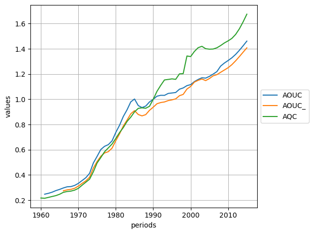
[231]:
<Axes: xlabel='periods', ylabel='values'>
Execute Identities
To execute an identity, use the execute() method of the identities workspace:
[232]:
identities.load(f"{SAMPLE_DATA_DIR}/fun.idt")
variables.load(f"{SAMPLE_DATA_DIR}/fun.var")
print(identities["GAP_"])
print(identities["GAP2"])
# reset variables GAP_ and GAP2
variables["GAP_"] = 0.
variables["GAP2"] = 0.
variables["GAP_;GAP2"]
Loading C:\soft\miniconda3\Lib\site-packages\iode\tests\data/fun.idt
48 objects loaded
Loading C:\soft\miniconda3\Lib\site-packages\iode\tests\data/fun.var
394 objects loaded
100*((QAF_/Q_F)-1)
100*(QAFF_/(Q_F+Q_I))
[232]:
Workspace: Variables
nb variables: 2
filename: c:\soft\miniconda3\Lib\site-packages\iode\tests\data\fun.var
description: Modèle fun - Simulation 1
sample: 1960Y1:2015Y1
mode: LEVEL
name 1960Y1 1961Y1 1962Y1 1963Y1 1964Y1 1965Y1 ... 2009Y1 2010Y1 2011Y1 2012Y1 2013Y1 2014Y1 2015Y1
GAP2 0.00 0.00 0.00 0.00 0.00 0.00 ... 0.00 0.00 0.00 0.00 0.00 0.00 0.00
GAP_ 0.00 0.00 0.00 0.00 0.00 0.00 ... 0.00 0.00 0.00 0.00 0.00 0.00 0.00
[233]:
# compute GAP_ and GAP2 (assuming Scalars and Variables are already loaded)
identities.execute("GAP_;GAP2")
variables["GAP_;GAP2"]
[233]:
Workspace: Variables
nb variables: 2
filename: c:\soft\miniconda3\Lib\site-packages\iode\tests\data\fun.var
description: Modèle fun - Simulation 1
sample: 1960Y1:2015Y1
mode: LEVEL
name 1960Y1 1961Y1 1962Y1 1963Y1 1964Y1 1965Y1 ... 2009Y1 2010Y1 2011Y1 2012Y1 2013Y1 2014Y1 2015Y1
GAP2 96.93 97.40 98.37 97.71 100.88 100.63 ... 100.85 100.54 101.36 102.19 102.50 102.15 101.59
GAP_ -3.20 -3.98 -2.12 -2.65 -0.23 -0.65 ... 1.96 1.61 2.61 3.61 4.06 3.78 3.24
[234]:
# compute GAP_ and GAP2 over a subset of the sample
variables["GAP_"] = 0.
variables["GAP2"] = 0.
identities.execute("GAP_;GAP2", "2000Y1", "2005Y1")
variables["GAP_;GAP2", "1998Y1:2007Y1"]
[234]:
Workspace: Variables
nb variables: 2
filename: c:\soft\miniconda3\Lib\site-packages\iode\tests\data\fun.var
description: Modèle fun - Simulation 1
sample: 1998Y1:2007Y1
mode: LEVEL
name 1998Y1 1999Y1 2000Y1 2001Y1 2002Y1 2003Y1 2004Y1 2005Y1 2006Y1 2007Y1
GAP2 0.00 0.00 104.61 103.06 102.17 102.82 104.47 104.36 0.00 0.00
GAP_ 0.00 0.00 4.51 3.31 2.62 3.46 5.48 5.58 0.00 0.00
Arithmetic Operations On Variables
[235]:
# reload variables to start from a clean state
variables.load(f"{SAMPLE_DATA_DIR}/fun.var")
# select a subset of variables for the examples below
vars_subset = variables["A*", "1991Y1:1995Y1"]
vars_subset
Loading C:\soft\miniconda3\Lib\site-packages\iode\tests\data/fun.var
394 objects loaded
[235]:
Workspace: Variables
nb variables: 5
filename: c:\soft\miniconda3\Lib\site-packages\iode\tests\data\fun.var
description: Modèle fun - Simulation 1
sample: 1991Y1:1995Y1
mode: LEVEL
name 1991Y1 1992Y1 1993Y1 1994Y1 1995Y1
ACAF 26.24 30.16 34.66 8.16 -13.13
ACAG -30.93 -40.29 -43.16 -16.03 -41.85
AOUC 1.02 1.03 1.03 1.05 1.05
AOUC_ 0.96 0.97 0.98 0.99 1.00
AQC 1.06 1.11 1.15 1.16 1.16
With a float
[236]:
# add a scalar to all values of a subset of variables
new_vars_subset = vars_subset + 2.0
new_vars_subset
[236]:
Workspace: Variables
nb variables: 5
filename: c:\soft\miniconda3\Lib\site-packages\iode\tests\data\fun.var
description: Modèle fun - Simulation 1
sample: 1991Y1:1995Y1
mode: LEVEL
name 1991Y1 1992Y1 1993Y1 1994Y1 1995Y1
ACAF 28.24 32.16 36.66 10.16 -11.13
ACAG -28.93 -38.29 -41.16 -14.03 -39.85
AOUC 3.02 3.03 3.03 3.05 3.05
AOUC_ 2.96 2.97 2.98 2.99 3.00
AQC 3.06 3.11 3.15 3.16 3.16
Between (Subsets Of) Variables Objects
[237]:
# add two subsets of variables
new_vars_subset = vars_subset + vars_subset
new_vars_subset
[237]:
Workspace: Variables
nb variables: 5
filename: c:\soft\miniconda3\Lib\site-packages\iode\tests\data\fun.var
description: Modèle fun - Simulation 1
sample: 1991Y1:1995Y1
mode: LEVEL
name 1991Y1 1992Y1 1993Y1 1994Y1 1995Y1
ACAF 52.48 60.32 69.32 16.32 -26.26
ACAG -61.87 -80.57 -86.32 -32.06 -83.69
AOUC 2.05 2.06 2.06 2.09 2.10
AOUC_ 1.93 1.95 1.96 1.98 1.99
AQC 2.13 2.22 2.31 2.31 2.32
With pandas Series or DataFrame
See the Arithmetic Operations On Variables With pandas Series And DataFrames section from the IODE and pandas tutorial for more details.
With larray Arrays
See the Arithmetic Operations On Variables With larray Array objects section from the IODE and larray tutorial for more details.
With numpy ndarrays
See the Arithmetic Operations On Variables With numpy ndarray objects section from the IODE and numpy tutorial for more details.
Estimation
To estimate either one equation or a block of equations, use the estimate method of the Equation class or the estimate method of the Equations workspace:
Calling the estimate(from_period, to_period, list_eqs, quiet) method estimates an equation or a block of equations in the specified periods range.
At the end of the estimation process, certain variables and scalars are automatically created if the process has converged. These variables and scalars can be used for computational purposes and, as they are part of the global workspace, can be saved for future use.
The tests resulting from the last estimation are saved as scalars. The same applies to residuals, left-hand and right-hand members of equations.
Saved tests (as scalars) have the following names (e<ith>_* for the equation of the block):
e<ith>_n: number of sample periodse<ith>_k: number of estimated coefficientse<ith>_stdev: std dev of residualse<ith>_meany: mean of Ye<ith>_ssres: sum of squares of residualse<ith>_stderr: std errore<ith>_stderrp: std error percent (in %)e<ith>_fstat: F-State<ith>_r2: R squaree<ith>_r2adj: adjusted R-squarede<ith>_dw: Durbin-Watsone<ith>_loglik: Log Likelihood
Calculated series are saved in special variables:
_YCALC<i>: right-hand side of the equation in the block_YOBS<i>: left-hand side of the equation in the block_YRES<i>: residuals of the equation of the block
Outside the estimation sample, the series values are NA.
Let’s start by reloading all workspaces:
[238]:
comments.load(f"{SAMPLE_DATA_DIR}/fun.cmt")
equations.load(f"{SAMPLE_DATA_DIR}/fun.eqs")
identities.load(f"{SAMPLE_DATA_DIR}/fun.idt")
lists.load(f"{SAMPLE_DATA_DIR}/fun.lst")
scalars.load(f"{SAMPLE_DATA_DIR}/fun.scl")
tables.load(f"{SAMPLE_DATA_DIR}/fun.tbl")
variables.load(f"{SAMPLE_DATA_DIR}/fun.var")
Loading C:\soft\miniconda3\Lib\site-packages\iode\tests\data/fun.cmt
317 objects loaded
Loading C:\soft\miniconda3\Lib\site-packages\iode\tests\data/fun.eqs
274 objects loaded
Loading C:\soft\miniconda3\Lib\site-packages\iode\tests\data/fun.idt
48 objects loaded
Loading C:\soft\miniconda3\Lib\site-packages\iode\tests\data/fun.lst
17 objects loaded
Loading C:\soft\miniconda3\Lib\site-packages\iode\tests\data/fun.scl
161 objects loaded
Loading C:\soft\miniconda3\Lib\site-packages\iode\tests\data/fun.tbl
46 objects loaded
Loading C:\soft\miniconda3\Lib\site-packages\iode\tests\data/fun.var
394 objects loaded
Example for one equation:
[239]:
# ---- estimate coefficients of one equation ----
print(f"ACAF equation LEC: {equations['ACAF'].lec}")
print(f"ACAF equations coefficients (= scalars): {equations['ACAF'].coefficients}")
print(f"ACAF equations variables: {equations['ACAF'].variables}")
# copy the original values of the coefficients into an isolated scalars workspace
# Useful to restore the original values if the estimation process didn't go well
scalars_copy = scalars[equations['ACAF'].coefficients].copy()
print(f"scalars names in scalars_copy: {scalars_copy.names}")
# reset scalars
for name in equations['ACAF'].coefficients:
scalars[name] = 0., 1.
# estimate the 'ACAF' equation for the periods ranging from '1980Y1' to '1996Y1'
success = equations.estimate("1980Y1", "1996Y1", "ACAF")
# or equivalently
success = equations["ACAF"].estimate("1980Y1", "1996Y1")
print(f"Equation estimation success: {success}")
print(f"Resulting values for the coefficient 'acaf1': {scalars['acaf1']}")
print(f"Resulting values for the coefficient 'acaf2': {scalars['acaf2']}")
print(f"Resulting values for the coefficient 'acaf4': {scalars['acaf4']}")
ACAF equation LEC: (ACAF/VAF[-1]) :=acaf1+acaf2*GOSF[-1]+
acaf4*(TIME=1995)
ACAF equations coefficients (= scalars): ['acaf1', 'acaf2', 'acaf4']
ACAF equations variables: ['ACAF', 'VAF', 'GOSF', 'TIME']
scalars names in scalars_copy: ['acaf1', 'acaf2', 'acaf4']
Estimating : iteration 1 (||eps|| = 0.173205)
Estimating : iteration 2 (||eps|| = 5.16075e-09)
Solution reached after 2 iteration(s). Creating results file ...
Estimating : iteration 1 (||eps|| = 7.05003e-13)
Solution reached after 1 iteration(s). Creating results file ...
Equation estimation success: True
Resulting values for the coefficient 'acaf1': Scalar(0.0157705, 1, 0.00136949)
Resulting values for the coefficient 'acaf2': Scalar(-7.96505e-06, 1, 1.48247e-06)
Resulting values for the coefficient 'acaf4': Scalar(-0.0085027, 1, 0.00208257)
Example for a block of equations:
[240]:
# ---- estimate a block of equations ----
print(f"ACAF equation LEC: {equations['ACAF'].lec}")
print(f"ACAF equations coefficients (= scalars): {equations['ACAF'].coefficients}")
print(f"ACAF equations variables: {equations['ACAF'].variables}")
print(f"DPUH equation LEC: {equations['DPUH'].lec}")
print(f"DPUH equations coefficients (= scalars): {equations['DPUH'].coefficients}")
print(f"DPUH equations variables: {equations['DPUH'].variables}")
# copy the original values of the coefficients into an isolated scalars workspace
# Useful to restore the original values if the estimation process didn't go well
scalars_names = equations['ACAF'].coefficients + equations['DPUH'].coefficients
scalars_names = list(set(scalars_names)) # removed duplicates
scalars_copy = scalars[scalars_names].copy()
print(f"scalars names in scalars_copy: {scalars_copy.names}")
# reset scalars
for name in equations['ACAF'].coefficients:
scalars[name] = 0., 1.
for name in equations['DPUH'].coefficients:
scalars[name] = 0., 1.
# prepare equations (same block and method)
block = "ACAF;DPUH"
for name in block.split(";"):
equations[name] = {"block": block, "method": "LSQ"}
# estimation the block 'ACAF;DPUH' for the periods ranging from '1980Y1' to '1996Y1'
success = equations.estimate("1980Y1", "1996Y1", block)
print(f"Block estimation success: {success}")
print(f"Resulting values for the coefficient 'acaf1': {scalars['acaf1']}")
print(f"Resulting values for the coefficient 'acaf2': {scalars['acaf2']}")
print(f"Resulting values for the coefficient 'acaf4': {scalars['acaf4']}")
print(f"Resulting values for the coefficient 'dpuh_1': {scalars['dpuh_1']}")
print(f"Resulting values for the coefficient 'dpuh_2': {scalars['dpuh_2']}")
ACAF equation LEC: (ACAF/VAF[-1]) :=acaf1+acaf2*GOSF[-1]+
acaf4*(TIME=1995)
ACAF equations coefficients (= scalars): ['acaf1', 'acaf2', 'acaf4']
ACAF equations variables: ['ACAF', 'VAF', 'GOSF', 'TIME']
DPUH equation LEC: dln (DPUH/DPUHO):=dpuh_1+dpuh_2*dln(IHU/PI5)+dln PC
DPUH equations coefficients (= scalars): ['dpuh_1', 'dpuh_2']
DPUH equations variables: ['DPUH', 'DPUHO', 'IHU', 'PI5', 'PC']
scalars names in scalars_copy: ['acaf1', 'acaf2', 'acaf4', 'dpuh_1', 'dpuh_2']
Estimating : iteration 1 (||eps|| = 0.223607)
Estimating : iteration 2 (||eps|| = 5.16075e-09)
Solution reached after 2 iteration(s). Creating results file ...
Estimating : iteration 1 (||eps|| = 4.38565e-12)
Solution reached after 1 iteration(s). Creating results file ...
Block estimation success: True
Resulting values for the coefficient 'acaf1': Scalar(0.0157705, 1, 0.00136079)
Resulting values for the coefficient 'acaf2': Scalar(-7.96505e-06, 1, 1.47188e-06)
Resulting values for the coefficient 'acaf4': Scalar(-0.0085027, 1, 0.00206603)
Resulting values for the coefficient 'dpuh_1': Scalar(0.0109855, 1, 0.00481857)
Resulting values for the coefficient 'dpuh_2': Scalar(0.0574893, 1, 0.0368951)
Simulation
To simulate a model, you must create and initialize an instance of the Simulation class.
Models
IN IODE, a model is simply a list of equations. No other construction is necessary: in this way, to modify a model, the only thing to do is to modify the list that defines it. For example, if a model is logically divided into 5 blocks, 5 lists of equations will be defined:
BLOC1 : A, B, C, D
BLOC2 : X, Y
BLOC3 : C1, C2, C3, C4
BLOC4 : X_A1, X_A2, X_A3
BLOC5 : R1, R2, R3, S_12
MODSIM : $BLOC1, $BLOC2, $BLOC3, $BLOC4, $BLOC5
To simulate a model, all equations of the model must have been loaded or created. In addition, all the variables and scalars used in the model equations must have been loaded or created. Values of exogenous variables and of scalar cannot be NA (Not Available) over the simulation periods.
Exchange Endo-Exo
It is possible to set endogenous-exogenous pairs for goal seeking. For each pair, the status of the variables is exchanged: endogenous becomes exogenous and vice versa. This enables the model to be run through known endogenous values and to deduce the necessary values for the associated exogenous variables. The exogenous variables take on the value calculated over the entire workspace period. See the documentation of the
model_exchange method.
Newton-Raphson Algorithm
When an equation is not explicitly defined in terms of its endogen, or when the endogen appears several times in the equation, the simulation algorithm tries to solve the equation using a Newton method. If this method fails, a secant method is used to find a solution to the equation. However, there is no guarantee that a solution will be found in every case. Non-continuous functions (singularities) such as:
may be impossible to solve around their singular point. For this type of problem, the only solution is to modify the form of the equation:
Warning:
As the endogenous variable of an equation carries the name of the equation, it is not possible to place in a model two equations with the same endogenous variable.
The order in which equations are introduced in the lists can influence the behavior of the simulation algorithm. As this is a Gauss-Seidel algorithm, the information calculated is used directly in the rest of the calculation. If X depends on Y, it’s better to place Y before X in the list of equations.
Examples
[241]:
from iode import SimulationSort
print(f"possible sort algorithms: {[member.name for member in SimulationSort]}")
possible sort algorithms: ['CONNEX', 'BOTH', 'NONE']
[242]:
from iode import SimulationInitialization
print(f"possible initialization methods: {[member.name for member in SimulationInitialization]}")
possible initialization methods: ['TM1', 'TM1_A', 'EXTRA', 'EXTRA_A', 'ASIS', 'TM1_NA', 'EXTRA_NA']
[243]:
from iode import Simulation
# create and initialize a Simulation instance
simu = Simulation(sort_algorithm=SimulationSort.BOTH, initialization_method=SimulationInitialization.TM1)
print(simu)
--- Simulation ---
convergence_threshold = 0.001
relax = 1.0
max_nb_iterations = 100
sort_algorithm = BOTH (Connex compon. + Triangulation)
initialization_method = TM1 (Y := Y[-1], if Y null or NA)
debug = False
nb_passes = 5
debug_newton = False
------------------
To run the simulation, call the Simulation.model_simulate method:
[244]:
print(f"exogenous variable 'UY': {equations['UY'].lec}")
print(f"endogenous variable 'XNATY': {identities['XNATY']}")
# reset values of exogenous variable
variables["UY", "2000Y1:2015Y1"] = 0.0
print(f"exogenous variable 'UY' before simulation:\n{variables['UY', '1998Y1:2005Y1']}")
# run the simulation for the periods range '2000Y1' to '2015Y1'
success = simu.model_simulate("2000Y1", "2015Y1", quiet=True)
print(f"Simulation success: {success}")
print(f"exogenous variable 'UY' after simulation:\n{variables['UY', '1998Y1:2005Y1']}")
exogenous variable 'UY': UY := NATY-NDOMY-NIY-NGY-(EFXY-EFMY)-NFY
endogenous variable 'XNATY': grt NATY
exogenous variable 'UY' before simulation:
Workspace: Variables
nb variables: 1
filename: c:\soft\miniconda3\Lib\site-packages\iode\tests\data\fun.var
description: Modèle fun - Simulation 1
sample: 1998Y1:2005Y1
mode: LEVEL
name 1998Y1 1999Y1 2000Y1 2001Y1 2002Y1 2003Y1 2004Y1 2005Y1
UY 671.46 647.39 0.00 0.00 0.00 0.00 0.00 0.00
Simulation success: True
exogenous variable 'UY' after simulation:
Workspace: Variables
nb variables: 1
filename: c:\soft\miniconda3\Lib\site-packages\iode\tests\data\fun.var
description: Modèle fun - Simulation 1
sample: 1998Y1:2005Y1
mode: LEVEL
name 1998Y1 1999Y1 2000Y1 2001Y1 2002Y1 2003Y1 2004Y1 2005Y1
UY 671.46 647.39 624.18 645.05 661.61 676.56 680.90 682.99
Import/Export IODE workspaces from/to pandas Series and DataFrame
To import / export the content of the comments, identities and lists workspaces from/to a pandas Series object, use the from_series() and to_series() methods.
Alternatively, you can use the series property to export the content of the comments, identities and lists workspaces to a pandas Series object.
For the examples, see the pandas tutorial.
Import/Export IODE Variables workspace from/to numpy ndarray
To import / export the content of the Variables workspace (or a subset of it) from/to a numpy ndarray object, use the from_numpy and to_numpy methods.
For the examples, see the numpy tutorial.
Import/Export the Variables workspace from/to LArray Array
To import / export the content of the variables workspaces from/to an LArray Array object, use the from_array() and to_array() methods.
For the examples, see the larray tutorial.
Execute IODE report commands/files
To run an IODE command, use the execute_command() function:
[245]:
from iode import execute_command
# ---- execute IODE commands ----
print("Execute IODE commands (useful for IODE functions and commands not yet ported to Python):")
execute_command("$WsClearVar")
execute_command("$WsSample 2000Y1 2005Y1")
execute_command("$DataCalcVar A t+1")
execute_command("$DataCalcVar B t-1")
execute_command("$DataCalcVar C A/B")
execute_command("$DataCalcVar D grt A")
execute_command("$WsSaveVar test_var.av")
with open("test_var.av", "r") as f:
print(f.read())
Execute IODE commands (useful for IODE functions and commands not yet ported to Python):
iode> $WsClearVar
iode> $WsSample 2000Y1 2005Y1
iode> $DataCalcVar A t+1
iode> $DataCalcVar B t-1
iode> $DataCalcVar C A/B
iode> $DataCalcVar D grt A
iode> $WsSaveVar test_var.av
Saving test_var.av
sample 2000Y1 2005Y1
A 1 2 3 4 5 6
B -1 0 1 2 3 4
C -1 na 3 2 1.66666666666667 1.5
D na 100 50 33.3333333333333 25 20
To run an entire IODE report (i.e. file with the ‘.rep’ extension), call the execute_report() function:
[246]:
from iode import execute_report
# ---- execute IODE reports ----
print("Execute an IODE report -> execute_report()")
with open("create_var.rep", "w") as f:
f.write("$WsClearVar\n")
f.write("$WsSample 2000Y1 2005Y1\n")
f.write("$DataCalcVar %1% t+1 \n")
f.write("$DataCalcVar %2% t-1 \n")
f.write("$DataCalcVar %3% %1%/%2%\n")
f.write("$DataCalcVar %4% grt %1% \n")
f.write("$WsSaveVar test_var.av\n")
execute_report("create_var.rep", ["A", "B", "C", "D"])
with open("test_var.av", "r") as f:
print(f.read())
Execute an IODE report -> execute_report()
iode> $WsClearVar
iode> $WsSample 2000Y1 2005Y1
iode> $DataCalcVar A t+1
iode> $DataCalcVar B t-1
iode> $DataCalcVar C A/B
iode> $DataCalcVar D grt A
iode> $WsSaveVar test_var.av
Saving test_var.av
sample 2000Y1 2005Y1
A 1 2 3 4 5 6
B -1 0 1 2 3 4
C -1 na 3 2 1.66666666666667 1.5
D na 100 50 33.3333333333333 25 20
Graphical User Interface
It is possible to run the graphical user interface to view the content of the IODE workspace from any line of a Python script. Simply call the function view_workspace() to open the GUI.
Content of a Python script:
from iode import view_workspace, ...
... code here ...
# To view the workspace, you can use the following command:
view_workspace()
# To open the graphical user interface showing the files
# from a specific directory, pass the path to the directory
# as an argument:
view_workspace("path/to/your/directory")
... code here ...